Introduction

This page hosts documentations and specifications for some of the cryptographic algorithms of Mina. For the Rust documentation, see here.

Note that this book is a work in progress, not necessarily reflecting the current state of Mina.

Authors: Izaak Meckler, Vanishree Rao, Matthew Ryan, Anaïs Querol, Joseph Spadavecchia, David Wong, Xiang Xie

In memory of Vitaly Zelov.

Terminology

This document is intended primarily to communicate mathematical ideas to programmers with some experience of math.

To that end, we will often be ambivalent about the difference between sets and types (in whatever programming language, but usually I am imagining some idealized form of Rust or OCaml). So for example we may write

$A$ is a type
$A$ is a set
A is a type

and these should all be interpreted the same way, assuming it makes sense in the context. Similarly, we may write either of the following, and potentially mean the same thing:

$a : A$
$a \in A$
a : A

We use

$\to$ for function types
$\mapsto$ for defining functions

Also, we usually assume functions are computed by a program (in whatever sense of “program” makes sense in the given context). So if we say “let $f : A \to B$ ”, we typically mean that

$A$ and $B$ are types in some programming language which makes sense in the context (or maybe that they are sets, again depending on context)
$f$ is actually a program computing a function of the type $A \to B$ (again, in whatever sense of program makes sense in context)

Groups

Groups are an algebraic structure which

are used in most widely deployed signature schemes
are used in most widely deployed zk-SNARKs
generalize the notion of a collection of symmetries of an object
generalize certain aspects of numbers

I will not touch on the last two too much.

First let’s do a quick definition and then some examples.

Definition. A group is a set $G$ with a binary operation $* : G \times G \to G$ , an identity $e \in G$ for that operation, and an inverse map $()^{- 1} : G \to G$ such that

$*$ is associative: $x * (y * z) = (x * y) * z$ for all $x, y, z$ .
$e$ is an identity for $*$ . I.e., $e * x = x * e = x$ for all $x$ .
$()^{- 1}$ is an inverse map for $*$ with identity $e$ . I.e., $x * x^{- 1} = x^{- 1} * x = e$ for all $x$ .

So basically, an invertible binary operation. Definition in hand, we can see some examples:

The integers $Z$ with $+$ , $0$ as identity, and negation as inverse.
For any natural number $n$ , the integers mod $n$ . This can be thought of as the set of numbers ${0, \dots, n - 1}$ with the operation being $+$ followed by taking remainder mod $n$ . It can also be thought of as the group of rotations of an $n$ -gon.
For any set $X$ , the set of invertible functions $X \to X$ (a.k.a permutations) with function composition as the operation, the identity function as the identity, and function inverse as the inverse operation.
The set of translations of a plane $R \times R$ with composition of translations (since the composition of translations is a translation). The identity is translating by $(0, 0)$ and inverse is reversing the translation. This is equivalent to the group $R \times R$ with coordinate-wise addition as the operation and coordinate-wise negation as the inverse.
The set of rotations of a sphere with composition as the operation, doing nothing as the identity, and performing the rotation in reverse as the inverse map.
For any field $F$ , the set $F^{\times} := F ∖ {0}$ , with field multiplication as the operation, $1$ as the identity, and $x \mapsto 1/ x$ as the inverse map. This is called the group of units of $F$ .

Sometimes, instead of $x * y$ we simply write $x y$ when $*$ is clear from context.

Abelian groups

An abelian group is a group in which $*$ is commutative, meaning $x * y = y * x$ . Typically, in that case, we write the group operation as $+$ instead and we write the identity as $0$ .

Some examples are

the integers with addition
the integers mod $n$ with addition
the group of units of a field $F$
the real numbers with addition
the rational numbers with addition
the real numbers with multiplication
the rational numbers with multiplication
vectors of integers of some fixed dimension with coordinate-wise addition
The set of polynomials over a ring $R$ , $R [x]$ with addition

Abelian groups are equivalently described as what are called $Z$ -modules. A $Z$ -module is like a vector space, but with the integers instead of a field.

Basically a $Z$ -module (or equivalently an Abelian group) is a structure where you can add elements and where it makes sense to multiply a group element by an integer.

If $G$ is an abelian group, we can define this “multiplication by an integer” as follows. If $n \geq 0$ , then for $g \in G$ , we can define $n \cdot g$ by

$n \cdot g := n g + \dots + g$

and if $n < 0$ , then define $n \cdot g := ∣ n ∣ \cdot (- g)$ . Or equivalently.,

$n \cdot g = ∣ n ∣ (- g) + \dots + (- g) = - ∣ n ∣ g + \dots + g$

This is the general sense of what is called scalar-multiplication or sometimes exponentiation in cryptography.

Cyclic groups

A cyclic group $G$ is a special kind of abelian group. It is an abelian group generated by a single element $g \in G$ . That is, a cyclic group $G$ (generated by $g \in G$ ) is one in which for every $h \in G$ we have $h = n g$ for some $n \in Z$ .

Groups in cryptography

Many cryptographic protocols are defined generically with respect to any abelian group that has a “hard discrete log”.

Let

$G$ be a cyclic group
$g$ a generator of $G$
$μ$ a probability distribution on $G$
$A$ a set of algorithms of type $G \to Z$ with runtime and memory usage bounds. In other words, a set of tuples $(P, t, m)$ where $P$ is a program of type $G \to Z$ , $t$ is a bound on the time that program can be run, and $m$ is a bound on the amount of memory that program can use.

In practice you fix this to be something like, the set of all computations that can be run for less than 1 trillion $.
$ε \in [0, 1]$ a probability, usually taken to be something close to 0 like $1/ 2^{128}$

Then we can define the $(G, g, μ, A, ε)$ -computational discrete-log assumption which says:

For any $(P, t, m) \in A$ , if you sample h from G according to $μ$ , then the probability that $P (h) \cdot h = g$ is smaller than $ε$ , assuming $P$ successfully runs within the given resource bounds.

Sometimes this is called the computational Diffie–Helman assumption. Basically what it’s saying is that for a group element $h$ sampled randomly, you can’t practically compute how many times you have to add $g$ to itself to get $h$ .

Another really important assumption is the no-relation assumption (TODO: name).

Basically what this says is that randomly selected group elements have no efficiently computable linear relations between them. Formally, letting $G$ be a group and $μ$ a probability distribution on $G$ , and $A$ a set of programs (with resource bounds) that take in a list of group elements as inputs and outputs a list of integers of the same length.

Then the $(G, μ, A, N, ε)$ -no-relation assumption says for all $(P, t, m) \in A$ , for any $n \leq N$ , if you sample $g_{1}, \dots, g_{n}$ according to $μ$ , letting $[e_{1}, \dots, e_{n}] = P ([g_{1}, \dots, g_{n}])$ , it is not the case that

$e_{1} \cdot g_{1} + \dots + e_{n} \cdot g_{n} = 0$

except with probability $ε$ (assuming program $P$ runs in time $t$ with memory $m$ ).

Generic group model

Elliptic curves

Now, what are some concrete groups that we can safely make the no-relation or computational discrete log hardness assumptions about?

Well, the most efficiently implementable groups that people have come up with – and that we believe satisfy the above assumptions for $A$ being the class of realistic computations and $ε$ being something like $1/ 2^{128}$ – are elliptic curves over finite fields.

Giving a complete definition of what an elliptic curve is requires a lot of math, and is not very useful from the point of view of cryptography. So we will give a definition that is not complete, but more useful.

An elliptic curve $E$ over a field $F$ is a set of the form

${(x, y) \in F \times F ∣ y^{2} = x^{3} + a x + b}$

for some $a, b \in F$ , plus an additional point $O$ which is called the point at infinity. Basically it’s a set of pairs satisfying some equation of that form. The data of the elliptic curve itself is just the field $F$ together with the constants $a$ and $b$ .

What is special about elliptic curves is that there is a way of giving them a group structure with simple to compute operations that we believe satisfy the hardness assumptions described above.

Group negation $(-) : E \to E$ is defined by

$- (x_{0}, y_{0}) = (x_{0}, - y_{0})$

so we just negate the $y$ coordinate.

The identity for the group is $O$ , the point at infinity. For that point we may also therefore write it as $0$ .

Group addition is more complicated to define, so we will not, but here is what’s worth knowing about how to compute $(x_{0}, y_{0}) + (x_{1}, y_{1})$

There are three cases
1. $x_{0} \neq = x_{1}$
2. $x_{0} = x_{1}$ and $y_{0} = y_{1}$
3. $x_{0} = x_{1}$ but $y_{0} \neq = y_{1}$ . In this case it turns out $y_{0} = - y_{1}$ and so the two points are inverse, and we return $O$
In cases 1 and 2, the algorithm to compute the result just performs a simple sequence of some field operations (multiplications, additions, divisions, subtractions) with the input values. In other words, there is a simple arithmetic formula for computing the result.

Elliptic curves in Rust

Elliptic curves in Sage

Serializing curve points

Given a curve point $(x, y)$ we know $y^{2} = x^{3} + a x + b$ and thus $y$ is one of the two square roots of $x^{3} + a x + b$ . If $y$ is a given square root, the other square root is $- y$ since $y^{2} = (- y)^{2}$ . So, if we know $x$ , then we almost know the whole curve point: we just need a single bit to tell us which of the two possible values (i.e., the two square roots of $x^{3} + a x + b$ ) is the y coordinate.

Here is how this is commonly done over prime order fields $F_{p}$ , assuming $p \neq = 2$ . Remember that we represent elements of $F_{p}$ as integers in the range $[0, p - 1]$ . In this representation, for a field element $y$ , $- y$ is the integer $p - y$ (or $0$ if $y = 0$ ). Thus, if $y$ is odd, then $- y$ is even (since $p$ is odd and an odd minus an odd is even). Similarly, if $y$ is even, then $- y$ is odd (since an odd minus an even is odd).

So, for any $y$ , unless $y$ is 0, $y$ and $- y$ have opposite parities. Parity can easily be computed: it’s just the least significant bit. Thus, we have an easy way of encoding a curve point $(x, y)$ . Send

$x$ in its entirety
The least significant bit $b_{0}$ of $y$

Given this, we can reconstruct $y$ as follows.

Compute any square root $Y$ of $x^{3} + a x + b$
If the least significant bit of $Y$ is equal to $b_{0}$ , then $y = Y$ , otherwise, $y = - Y$

In the case of Mina, our field elements require 255 bits to store. Thus, we can encode a curve point in $255 + 1 = 256$ bits, or 32 bytes. At the moment this optimized encoding is not implemented for messages on the network. It would be a welcome improvement.

Projective form / projective coordinates

The above form of representing curve points as pairs – which is called affine form – is sometimes sub-optimal from an efficiency perspective. There are several other forms in which curve points can be represented, which are called projective forms.

The simple projective form represents a curve $E$ as above as the set

${(X, Y, Z) \in F^{3} ∣ (Y / Z)^{2} = (X / Z)^{3} + a (X / Z) + b}$

If you think about it, this is saying that $(X / Z, Y / Z)$ is a point on the original curve in affine form. In other words, in projective form we let the first two coordinates get scaled by some arbitrary scaling factor $Z$ , but we keep track of it as the third coordinate.

To be clear, this means curve points have many different representations. If $(x, y, z)$ is a curve point in projective coordinates, and $s$ is any element of $F$ , then $(s x, sy, sz)$ is another representation of the same curve point.

This means curve points require more space to store, but it makes the group operation much more efficient to compute, as we can avoid having to do any field divisions, which are expensive.

Jacobian form / Jacobian coordinates

There is another form, which is also sometimes called a projective form, which is known as the jacobian form. There, a curve $E$ would be represented as

${(X, Y, Z) \in F^{3} ∣ (X / Z^{2}, Y / Z^{3}) \in E}$

so the triple $(X, Y, Z)$ corresponds to the affine point $(X / Z^{2}, Y / Z^{3})$ . These are the fastest for computing group addition on a normal computer.

Take aways

Use affine coordinates when the cost of division doesn’t matter and saving space is important. Specific contexts to keep in mind:
- Working with elliptic curve points inside a SNARK circuit
Use Jacobian coordinates for computations on normal computers, or other circumstances where space usage is not that costly and division is expensive.
Check out this website for the formulas for implementing the group operation.

More things to know

When cryptographers talk about “groups”, they usually mean a “computational group”, which is a group equipped with efficient algorithms for computing the group operation and inversion. This is different because a group in the mathematical sense need not have its operations be computable at all.

Exercises

Implement a type JacobianPoint<F:Field> and functions for computing the group operation
Familiarize yourself with the types and traits in ark_ec. Specifically,
- todo
Implement fn decompress<F: SquareRootField>(c: (F, bool)) -> (F, F)

Rings

A ring is like a field, but where elements may not be invertible. Basically, it’s a structure where we can

add
multiply
subtract

but not necessarily divide. If you know what polynomials are already, you can think of it as the minimal necessary structure for polynomials to make sense. That is, if $R$ is a ring, then we can define the set of polynomials $R [x]$ (basically arithmetic expressions in the variable $x$ ) and think of any polynomial $f \in R [x]$ giving rise to a function $R \to R$ defined by substituing in for $x$ in $f$ and computing using $+$ and $\cdot$ as defined in $R$ .

So, in full, a ring $R$ is a set equipped with

$(+) : R \times R \to R$
$(\cdot) : R \times R \to R$
$(-) : R \to R$
$0 \in R$
$1 \in R$

such that

$(+, 0, -)$ gives the structure of an abelian group
$(\cdot)$ is associative and commutative with identity $1$
$+$ distributes over $\cdot$ . I.e., $x \cdot (y + z) = x \cdot y + x \cdot z$ for all $x, y, z$ .

Intro

The purpose of this document is to give the reader mathematical, cryptographic, and programming context sufficient to become an effective practitioner of zero-knowledge proofs and ZK-SNARKs specifically.

Some fundamental mathematical objects

In this section we’ll discuss the fundamental objects used in the construction of most ZK-SNARKs in use today. These objects are used extensively and without ceremony, so it’s important to understand them very well.

If you find you don’t understand something at first, don’t worry: practice is often the best teacher and in using these objects you will find they will become like the bicycle you’ve had for years: like an extension of yourself that you use without a thought.

Fields

A field is a generalization of the concept of a number. To be precise, a field is a set $F$ equipped with

An element $0 \in F$
An element $1 \in F$
A function $mul : F \times F \to F$
A function $add : F \times F \to F$
A function $sub : F \times F \to F$
A function $div : F \times (F ∖ {0}) \to F$

Note that the second argument to $div$ cannot be $0$ . We write these functions in the traditional infix notation writing

$x y$ or $x \cdot y$ for $mul (x, y)$
$x + y$ for $add (x, y)$
$x - y$ for $sub (x, y)$
$\frac{x}{y}$ for $div (x, y)$

and we also write $x^{- 1}$ for $div (1, x)$ and $- x$ for $sub (0, x)$ .

Moreover all these elements and functions must obey all the usual laws of arithmetic, such as

$x + (y + z) = (x + y) + z$
$x + y = y + x$
$x + (- x) = 0$
$x + 0 = x$
$x (yz) = (x y) z$
$x y = y x$
$\frac{x}{y} = z$ if and only if $x = zy$ , assuming $y \neq = 0$ .
$1 \cdot x = x$
$x (y + z) = x y + x z$

In short, $F$ should be an abelian group over $+$ with $0$ as identity and $sub (0, -)$ as inverse, $F ∖ {0}$ should be an abelian group over $\cdot$ with $1$ as identity and $div (1, -)$ as inverse, and addition should distribute over multiplication. If you don’t know what an abelian group is, don’t worry, we will cover it later.

The point of defining a field is that we can algebraically manipulate elements of a field the same way we do with ordinary numbers, adding, multiplying, subtracting, and dividing them without worrying about rounding, underflows, overflows, etc.

In Rust, we use the trait Field to represent types that are fields. So, if we have T : Field then values of type T can be multiplied, subtracted, divided, etc.

Examples

The most familiar examples of fields are the real numbers $R$ and the rational numbers $Q$ (ratios of integers). Some readers may also be friends with the complex numbers $C$ which are also a field.

The fields that we use in ZKPs, however, are different. They are finite fields. A finite field is a field with finitely many elements. This is in distinction to the fields $Q, R$ , and $C$ , which all have infinitely many elements.

What are finite fields like?

In this section we’ll try to figure out from first principles what a finite field should look like. If you just want to know the answer, feel free to skip to the next section.

Let’s explore what a finite field can possibly be like. Say $F$ is a finite field. If $n$ is a natural number like $4$ or $87$ we can imagine it as an element of $F$ by writing $n 1 + \dots + 1$ .

Since $F$ is finite it must be the case that we can find two distinct natural numbers $n < m$ which are the same when interpreted as elements of $F$ .

Then, $m - n = 0$ , which means the $F$ element $m - n 1 + \dots + 1$ is $0$ . Now that we have established that if you add $1$ to itself enough times you get $0$ , let $p$ be the least natural number such that if you add $1$ to itself $p$ times you get $0$ .

Now let’s show that $p$ is prime. Suppose it’s not, and $p = ab$ . Then since $p = 0$ in $F$ , $ab = 0$ . It is a fact about fields (exercise) that if $ab = 0$ then either $a$ is 0 or $b$ is 0. Either way, we would then get a natural number smaller than $p$ which is equal to $0$ in $F$ , which is not possible since $p$ is the smallest such number. So we have demonstrated that $p$ is prime.

The smallest number of times you have to add $1$ to itself to get 0 is called the characteristic of the field $F$ . So, we have established that every finite field has a characteristic and it is prime.

This gives us a big hint as to what finite fields should look like.

Prime order fields

With the above in hand, we are ready to define the simplest finite fields, which are fields of prime order (also called prime order fields).

Let $p$ be a prime. Then $F_{p}$ (pronounced “eff pee” or “the field of order p”) is defined as the field whose elements are the set of natural numbers ${0, 1, \dots, p - 1}$ .

$0$ is defined to be $0$
$1$ is defined to be $1$
$add (x, y) = (x + y) mod p$
$sub (x, y) = (x - y) mod p$
$mul (x, y) = (x \cdot y) mod p$
$div (x, y) = (x \cdot y^{p - 2}) mod p$

Basically, you just do arithmetic operations normally, except you take the remainder after dividing by $p$ . This is with the exception of division which has a funny definition. Actually, a more efficient algorithm is used in practice to calculate division, but the above is the most succinct way of writing it down.

If you want, you can try to prove that the above definition of division makes the required equations hold, but we will not do that here.

Let’s work out a few examples.

2 is a prime, so there is a field $F_{2}$ whose elements are ${0, 1}$ . The only surprising equation we have is

$1 + 1 = 0$

Addition is XOR and multiplication is AND.

Let’s do a more interesting example. 5 is a prime, so there is a field whose elements are ${0, 1, 2, 3, 4}$ . We have

$\frac{1}{2} = 1 \cdot 2^{5 - 2} = 2^{3} = 8 = 3$

where the last equality follows because everything is mod 5.

We can confirm that 3 is in fact $\frac{1}{2}$ by multiplying 3 and 2 and checking the result is 1.

$\frac{1}{2} \cdot 2 = 3 \cdot 2 = 6 = 1$

so that checks out.

In cryptography, we typically work with much larger finite fields. There are two ways to get a large finite field.

Pick a large prime $p$ and take the field $F_{p}$ . This is what we do in Mina, where we use fields in which $p$ is on the order of $2^{255}$ .
Take an extension of a small finite field. We may expand this document to talk about field extensions later, but it does not now.

Algorithmics of prime order fields

For a finite field $F_{p}$ where $p$ fits in $n$ bits (i.e., $p < 2^{n}$ ) we have

Addition, subtraction: $O (n)$
Multiplication $O (n^{2})$
Division $O (n^{2})$ I believe, in practice significantly slower than multiplication.

Actually, on a practical level, it’s more accurate to model the complexity in terms of the number of limbs rather than the number of bits where a limb is 64 bits. Asymptotically it makes no difference but concretely it’s better to think about the number of limbs for the most part.

As a result you can see it’s the smaller $n$ is the better, especially with respect to multiplication, which dominates performance considerations for implementations of zk-SNARKs, since they are dominated by elliptic curve operations that consist of field operations.

While still in development, Mina used to use a field of 753 bits or 12 limbs and now uses a field of 255 bits or 4 limbs. As a result, field multiplication became automatically sped up by a factor of $1 2^{2} / 4^{2} = 9$ , so you can see it’s very useful to try to shrink the field size.

Polynomials

The next object to know about is polynomials. A polynomial is a syntactic object that also defines a function.

Specifically, let $R$ be a field (or more generally it could even be a ring, which is like a field but without necessarily having division, like the integers $Z$ ). And pick a variable name like $x$ . Then $R [x]$ (pronounced, “R adjoin x” or “polynomials in x over R” or “polynomials in x with R coefficients”) is the set of syntactic expressions of the form

$a_{0} + a_{1} x + a_{2} x^{2} + \dots + a_{d} x^{d}$

where each $a_{i} \in R$ and $d$ is any natural number. If we wanted to be very formal about it, we could define $R [x]$ to be the set of lists of elements of $R$ (the lists of coefficients), and the above is just a suggestive way of writing that list.

An important fact about polynomials over $R$ is that they can be interpreted as functions $R \to R$ . In other words, there is a function $eval : R [x] \to (R \to R)$ defined by

$eval (a_{0} + a_{1} x + \dots + a_{d} x^{d}) = (y : R) \mapsto a_{0} + a_{1} y + \dots + a_{d} y^{d}$

where $x$ is just a variable name without a value assigned to it and $eval$ maps it to a field element $y$ and evaluates the function as the inner product between the list of coefficients and the powers of $y$ .

It is important to remember that polynomials are different than the functions that they compute. Polynomials are really just lists of coefficients. Over some fields, there are polynomials $p 1$ and $p 2$ such that $eval (p 1) = eval (p 2)$ , but $p 1 \neq = p 2$ .

For example, consider in $F_{2} [x]$ the polynomials $x$ and $x^{2}$ . These map to the same function $F_{2} \to F_{2}$ (meaning for $x \in R = F_{2} = {0, 1}$ it holds that $x = x^{2}$ ), but are distinct polynomials.

Some definitions and notation

If $f$ is a polynomial in $R [x]$ and $a \in R$ , we write $f (a)$ for $eval (f) (a)$

If $f$ is a polynomial, the degree of $f$ is the largest $d$ for which the coefficient of $x^{d}$ is non-zero in $f$ . For example, the degree of $x^{3} + 2 x^{10}$ is 10.

We will use the notation $R [x]_{< d}$ and $R [x]_{\leq d}$ for the set of polynomials of degree less-than and less-than-or-equal $d$ respectively.

Polynomials can be added (by adding the coefficients) and multiplied (by carrying out the multiplication formally and collecting like terms to reduce to a list of coefficients). Thus $R [x]$ is a ring.

Fundamental theorem of polynomials

An important fact for zk-SNARKs about polynomials is that we can use them to encode arrays of field elements. In other words, there is a way of converting between polynomials of degree $d$ and arrays of field elements of length $d + 1$ .

This is important for a few reasons

It will allow us to translate statements about arrays of field elements into statements about polynomials, which will let us construct zk-SNARKs.
It will allow us to perform certain operations on polynomials more efficiently.

So let’s get to defining and proving this connection between arrays of field elements.

The first thing to understand is that we won’t be talking about arrays directly in this section. Instead, we’ll be talking about functions $A \to F$ where $A$ is a finite subset of $F$ . The idea is, if $A$ has size $n$ , and we put an ordering on $A$ , then we can think of a function $A \to F$ as the same thing as an immutable array of length $n$ , since such a function can be thought of as returning the value of an array at the input position.

With this understanding in hand, we can start describing the “fundamental theorem of polynomials”. If $A \subseteq F$ has size $d + 1$ , this theorem will define an isomorphism between functions $A \to F$ and $F [x]_{\leq d}$ , the set of polynomials of degree at most $d$ .

Now let’s start defining this isomorphism.

One direction of it is very easy to define. It is none other than the evaluation map, restricted to $A$ :

$eval_{A} eval_{A} : F [x]_{\leq d} \to (A \to F) (c_{0} + \dots + c_{d} x^{d}) = a \mapsto i \leq d \sum c_{i} a^{i}$

We would now like to construct an inverse to this map. What would that mean? It would be a function that takes as input a function $φ : A \to F$ (remember, basically an array of length $∣ A ∣$ ), and returns a polynomial $f$ which agrees with $φ$ on the set $A$ . In other words, we want to construct a polynomial that interpolates between the points $(a, φ (a))$ for $a \in A$ .

Our strategy for constructing this polynomial will be straightforward. For each $a \in A$ , we will construct a polynomial $f_{a}$ that is equal to $φ (a)$ when evaluated at $a$ , and equal to $0$ when evaluated anywhere else in the set $A$ .

Then, our final polynomial will be $f := \sum_{a \in A} f_{a}$ . Then, when $f$ is evaluated at $a_{0} \in A$ , only the $f_{a_{0}}$ term will be non-zero (and equal to $φ (a_{0})$ as desired), all the other terms will disappear.

Constructing the interpolation map requires a lemma.

Lemma. (construction of vanishing polynomials)

Let $S \subseteq F$ . Then there is a polynomial $v_{S} \in F [x]$ of degree $∣ S ∣$ such that $v_{S}$ evaluates to $0$ on $S$ , and is non-zero off of $S$ . $v_{S}$ is called the vanishing polynomial of $S$ .

Proof. Let $v_{S} = \prod_{s \in S} (x - s)$ . Clearly $v_{S}$ has degree $∣ S ∣$ . If $t \in S$ , then $v_{S} (t) = 0$ since $x - t$ is one of the terms in the product defining $v_{S}$ , so when we evaluate at $t$ , $t - t = 0$ is one of the terms. If $t \in / S$ , then all the terms in the product are non-zero, and thus $v_{S} (t)$ is non-zero as well. $□$

Now we can define the inverse map. Define

$interp_{A} interp_{A} : (A \to F) \to F [x]_{\leq d} (f) = a \in A \sum \frac{f ( a )}{v _{A ∖ {a}} ( a )} \cdot v_{A ∖ {a}}$

Since each $v_{A ∖ {a}}$ has degree $d$ , this polynomial has degree $d$ . Now we have, for any $b \in A$ ,

$eval_{A} (interp_{A} (f)) (b) = a \in A \sum \frac{f ( a )}{v _{A ∖ {a}} ( a )} \cdot v_{A ∖ {a}} (b) = \frac{f ( b )}{v _{A ∖ {b}} ( b )} \cdot v_{A ∖ {b}} (b) + a \neq = b \sum \frac{f ( a )}{v _{A ∖ {a}} ( a )} \cdot v_{A ∖ {a}} (b) = f (b) + a \neq = b \sum \frac{f ( a )}{v _{A ∖ {a}} ( a )} \cdot 0 = f (b)$

Thus $eval_{A} \circ interp_{A}$ is the identity.

So we have successfully devised a way of interpolating a set of $d + 1$ points with a polynomial of degree $d$ .

What remains to be seen is that these two maps are inverse in the other direction. That is, that for any polynomial $f \in F [x]$ , we have

$interp_{A} (eval_{A} (f)) = f$

This says that if we interpolate the function that has the values of $f$ on $A$ , we get back $f$ itself. This essentially says that there is only one way to interpolate a set of $d + 1$ points with a degree $d$ polynomial. So let’s prove it by proving that statement.

Lemma: polynomials that agree on enough points are equal.

Let $F$ be a field and suppose $f, g \in F [x]$ have degree at most $d$ . Let $A \subseteq F$ have size $d + 1$ .

Suppose for all $a \in A$ , $f (a) = g (a)$ . Then $f = g$ as polynomials.

Proof. Define $h := f - g$ . Our strategy will be to show that $h$ is the zero polynomial. This would then imply that $f = g$ as polynomials. Note that $h$ vanishes on all of $A$ since $f$ and $g$ are equal on $A$ .

To that end, let $a \in A$ . Then we can apply the polynomial division algorithm to divide $h$ by $x - a$ and obtain polynomials $q_{a}, r_{a}$ such that $h = q_{a} (x - a) + r_{a}$ and $r_{a}$ has degree less than 1. I.e., $r_{a}$ is a constant in $F$ .

Now, $0 = h (a) = q_{a} (a) \cdot 0 + r_{a} = r_{a}$ so $r_{a} = 0$ and thus $h = q_{a} (x - a)$ .

Note that $q_{a}$ is 0 on all elements $b \in A$ with $b \neq = a$ since $h (b) = q_{a} (b) (b - a) = 0$ , but $b - a \neq = 0$ .

Thus, if we iterate the above, enumerating the elements of $A$ as $a_{0}, \dots, a_{d}$ , we find that $h = (x - a_{0}) q_{a_{0}} = (x - a_{0}) (x - a_{1}) q_{a_{1}} = \dots = (x - a_{0}) (x - a_{1}) \dots (x - a_{d}) q_{a_{d}}$

Now, if $q_{a_{d}}$ is not the zero polynomial, then $h$ will have degree at least $d + 1$ since it would have as a factor the $d + 1$ linear terms $(x - a_{i})$ . But since $f, g$ both have degree at most $d$ and $h = f - g$ , $h$ has degree at most $d$ as well. Thus, $q_{a_{d}} = 0$ , which means $h = 0$ as well.

This gives us the desired conclusion, that $f = g$ as polynomials. $□$

Now we can easily show that interpolating the evaluations of a polynomial yields that polynomial itself. Let $f \in F [x]_{\leq d}$ . Then $interp_{A} (eval_{A} (f))$ is a polynomial of degree at most $d$ that agrees with $f$ on $A$ , a set of size $d + 1$ . Thus, by the lemma, they are equal as polynomials. So indeed $interp_{A} (eval_{A} (f)) = f$ for all $f \in F [x]$ .

So far we have proven that $interp_{A}$ and $eval_{A}$ give an isomorphism of sets (i.e., a bijection) between the sets $A \to F$ and $F [x]_{\leq d}$ .

But we can take this theorem a bit further. The set of functions $A \to F$ can be given the structure of a ring, where addition and multiplication happen pointwise. I.e., for $f, g : A \to F$ we define $f + g := a \mapsto f (a) + g (a)$ and $f \cdot g := a \mapsto f (a) \cdot g (a)$ . Then we can strengthen our theorem to say

Fundamental theorem of polynomials (final version)

Let $d \in N$ and let $A \subseteq F$ with $∣ A ∣ = d + 1$ . With

$eval_{A} : F [x]_{\leq d} \to (A \to F) interp_{A} : (A \to F) \to F [x]_{\leq d}$

defined as above, these two functions define an isomorphism of rings.

That is is, they are mutually inverse and each one respects addition, subtraction and multiplication.

The fundamental theorem of polynomials is very important when it comes to computing operations on polynomials. As we will see in the next section, the theorem will help us to compute the product of degree $n$ polynomials in time $O (n lo g n)$ , whereas the naive algorithm takes time $O (n^{2})$ . To put this in perspective, if $n = 2^{16}$ , $n^{2}$ is $4096$ times larger than $n lo g n$ and the gap only gets bigger as $n$ grows.

Schwartz–Zippel lemma

Computer representation

There are three common representations for polynomials used in computer implementations.

Dense coefficient form. A degree $d$ polynomial is represented as a vector of length $d + 1$ of all the coefficients. Entry $i$ of the vector corresponds to the coefficient $a_{i}$ . This corresponds to the DensePolynomial type in arkworks. Sometimes this is also described as writing the polynomial “in the monomial basis”, because it amounts to writing the polynomial as a linear combination of the monomials $x^{i}$ .
Sparse coefficient form. If a polynomial does not have very many non-zero coefficients, the above representation is wasteful. In sparse coefficient form, you represent a polynomial as a vector (or potentially a hash-map) of pairs (usize, F) where F is the type of coefficients. The polynomial corresponding to the list [(i_0, b_0), ..., (i_n, b_n)] is $b_{0} x^{i_{0}} + \dots + b_{n} x^{i_{n}}$
Evaluation form. We fix an index set $A \subseteq F$ , with $A = {a_{0}, \dots, a_{d}}$ , and represent a polynomial $f \in F [x]_{\leq d}$ as the vector [f(a_0), ..., f(a_d)]. By the fundamental theorem of polynomials, this is a valid way of representing the polynomials, since the coefficients form can be obtained by using the $interp_{A}$ function.

The evaluation form is very important. The reason is that multiplying two polynomials in the evaluation form takes time $O (n)$ . You just multiply the two vectors entry-wise. By contrast, the coefficient forms naively require time $O (n^{2})$ to multiply.

Now, there is a trick. For certain sets $A \subseteq F$ , we can efficiently translate between the dense coefficients form and the evaluation form. That is, for certain $A$ , the functions $interp_{A}$ and $eval_{A}$ can be computed more efficiently than $O (n^{2})$ .

Multiplying polynomials

The algorithm that allows us to multiply polynomials in $O (n lo g n)$ is called the Cooley-Tukey fast Fourier transform, or FFT for short. It was discovered by Gauss 160 years earlier, but then separately rediscovered and publicized by Cooley-Tukey.

The heart of Cooley-Tukey FFT is actually about converting between coefficient and evaluation representations, rather than the multiplication itself. Given polynomials $p$ and $q$ in dense coefficient representation, it works like this.

Convert $p$ and $q$ from coefficient to evaluation form in $O (n lo g n)$ using Cooley-Tukey FFT
Compute $r = p * q$ in evaluation form by multiplying their points pairwise in $O (n)$
Convert $r$ back to coefficient form in $O (n lo g n)$ using the inverse Cooley-Tukey FFT

The key observation is that we can choose any $n$ distinct evaluation points to represent any degree $n - 1$ polynomial. The Cooley-Tukey FFT works by selecting points that yield an efficient FFT algorithm. These points are fixed and work for any polynomials of a given degree.

The next section describes the Cooley-Tukey FFT in detail.

Fast Fourier Transform (FFT)

This section describes how the Cooley-Tukey fast Fourier transform works. As we learned in the previous section, the key is to select evaluation points that yield an efficient FFT algorithm.

Specifically, say we have $ω \in F$ such that $ω^{n} = 1$ , and $ω^{r} \neq = 1$ for any $0 < r < n$ .

Put another way, all the values $1, ω, ω^{2}, ω^{3}, \dots, ω^{n - 1}$ are distinct and $ω^{n} = 1$ .

Put yet another way, the group generated by $ω$ inside $F^{\times}$ (written $⟨ ω ⟩$ ) has size $n$ .

We call such an $ω$ a primitive $n$ -th root of unity.

Suppose we have an $ω$ which is a primitive $2^{k}$ th root of unity and let $A_{k} = {1, ω, \dots, ω^{2^{k} - 1}}$ .

The FFT algorithm will let us compute $interp_{A_{k}}$ for this set.

Actually, it is easier to see how it will let us compute the $eval_{A_{k}}$ algorithm efficiently.

We will describe an algorithm $FFT (k, ω, f)$ that takes as input

$k \in N$
$ω \in F$ a primitive $2^{k}$ th root of unity
$f \in F [x]_{< 2^{k}}$ in dense coefficients form (i.e., as a vector of coefficients of length $n$ ).

and outputs the vector of evaluations $[f (1), f (ω), f (ω^{2}) \dots, f (ω^{2^{k} - 1})]$ and does it in time $O (k 2^{k})$ (which is to say, $n lo g n$ if $n = 2^{k}$ ).

Notice that naively, computing each evaluation $f (ω^{i})$ using the coefficients of $f$ would require time $O (n)$ , and so computing all $n$ of them would require time $O (n^{2})$ .

The algorithm $FFT (k, ω, f)$ can be defined recursively as follows.

If $k = 0$ , then $ω$ is a primitive $1$ st root of unity, and $f$ is a polynomial of degree $0$ . That means $ω = 1$ and also $f$ is a constant $c \in F$ . So, we can immediately output the array of evaluations $[c] = [f (1)]$ .

If $k > 0$ , then we will split $f$ into two polynomials, recursively call $FFT$ on them, and reconstruct the result from the recursive calls.

To that end, define $f_{0}$ to be the polynomial whose coefficients are all the even-index coefficients of $f$ and $f_{1}$ the polynomial whose coefficients are all the odd-index coefficients of $f$ . In terms of the array representation, this just means splitting out every other entry into two arrays. So that can be done in time $O (n)$ .

Write $f = \sum_{i < 2^{k}} c_{i} x^{i}$ , so that $f_{0} = \sum_{i < 2^{k - 1}} c_{2 i} x^{i}$ and $f_{1} = \sum_{i < 2^{k - 1}} c_{2 i + 1} x^{i}$ . Then

$f (x) = i < 2^{k} \sum c_{i} x^{i} = i < 2^{k - 1} \sum c_{2 i} x^{2 i} + i < 2^{k - 1} \sum c_{2 i + 1} x^{2 i + 1} = i < 2^{k - 1} \sum c_{2 i} (x^{2})^{i} + i < 2^{k - 1} \sum c_{2 i + 1} x \cdot (x^{2})^{i} = i < 2^{k - 1} \sum c_{2 i} (x^{2})^{i} + x i < 2^{k - 1} \sum c_{2 i + 1} (x^{2})^{i} = f_{0} (x^{2}) + x f_{1} (x^{2})$

Now, notice that if $ω$ is a $2^{k}$ th root of unity, then $ω^{2}$ is a $2^{k - 1}$ th root of unity. Thus we can recurse with $FFT (k - 1, ω^{2}, f_{0})$ and similarly for $f_{1}$ . Let

$[e_{0, 0}, \dots, e_{0, 2^{k - 1} - 1}] [e_{1, 0}, \dots, e_{1, 2^{k - 1} - 1}] = FFT (k - 1, ω^{2}, f_{0}) = FFT (k - 1, ω^{2}, f_{1})$

By assumption $e_{i, j} = f_{i} ((ω^{2})^{j})$ . So, for any $j$ we have

$f (ω^{j}) = f_{0} ((ω^{2})^{j}) + ω^{j} f_{1} ((ω^{2})^{j})$

Now, since $j$ may be larger than $2^{k - 1} - 1$ , we need to reduce it mod $2^{k - 1}$ , relying on the fact that if $τ$ is an $n$ th root of unity then $τ^{j} = τ^{j mod n}$ since $τ^{n} = 1$ . Thus, $(ω^{2})^{j} = (ω^{2})^{j mod 2^{k - 1}}$ and so we have

$f (ω^{j}) = f_{0} ((ω^{2})^{j mod 2^{k - 1}}) + ω^{j} f_{1} ((ω^{2})^{j mod 2^{k - 1}}) = e_{0, j mod 2^{k - 1}} + ω^{j} e_{1, j mod 2^{k - 1}}$

We can compute the array $W = [1, ω, \dots, ω^{2^{k} - 1}]$ in time $O (n)$ (since each entry is the previous entry times $ω$ ). Then we can compute each entry of the output in $O (1)$ as

$f (ω^{j}) = e_{0, j mod 2^{k - 1}} + W [j] \cdot e_{1, j mod 2^{k - 1}}$

There are $n$ such entries, so this takes time $O (n)$ .

This concludes the recursive definition of the algorithm $FFT (k, ω, f)$ .

Algorithm: computing $eval_{A_{k}}$

$Input f = [c_{0}, \dots, c_{2^{k} - 1}]$ the coefficients of polynomial $f (x) = \sum_{i < 2^{k}} c_{i} x^{i}$

$Compute W \leftarrow [1, ω, ω^{2}, \dots, ω^{2^{k} - 1}]$

$FFT (k, ω, f) \to [f (1), f (ω), f (ω^{2}) \dots, f (ω^{2^{k} - 1})]$

$if k == 0$

$return f$

$else$

$Compute f_{0} = [c_{0}, c_{2}, \dots, c_{2^{k} - 2}]$ the even coefficients of $f,$ corresponding to $f_{0} (x) = \sum_{i < 2^{k - 1}} c_{2 i} x^{i}$

$Compute f_{1} = [c_{1}, c_{3}, \dots, c_{2^{k} - 1}]$ the odd coefficients of $f,$ corresponding to $f_{1} (x) = \sum_{i < 2^{k - 1}} c_{2 i + 1} x^{i}$

$e_{0} \leftarrow FFT (k - 1, ω^{2}, f_{0})$

$e_{1} \leftarrow FFT (k - 1, ω^{2}, f_{1})$

$for j \in [0, 2^{k} - 1]$

$F_{j} \leftarrow e_{0, j mod 2^{k - 1}} + W [j] \cdot e_{1, j mod 2^{k - 1}}$

$return F$

Now let’s analyze the time complexity. Let $T (n)$ be the complexity on an instance of size $n$ (that is, for $n = 2^{k}$ ).

Looking back at what we have done, we have done

$O (n)$ for computing $f_{0}$ and $f_{1}$
two recursive calls, each of size $n /2$
$O (n)$ for computing the powers of $ω$
$O (n)$ for combining the results of the recursive calls

In total, this is $O (n) + 2 T (n /2)$ . Solving this recurrence yields $T (n) = O (n) \cdot l o g n = O (n lo g n)$ . Basically, there are $lo g n$ recursions before we hit the base case, and each step takes time $O (n)$ . $□$

Now, in practice there are ways to describe this algorithm non-recursively that have better concrete performance, but that’s out of scope for this document. Read the code if you are interested.

Using the FFT algorithm to compute $interp_{A_{k}}$

So far we have a fast way to compute $eval_{A_{k}} (f)$ all at once, where $A_{k}$ is the set of powers of a $2^{k}$ th root of unity $ω$ . For convenience let $n = 2^{k}$ .

Now we want to go the other way and compute a polynomial given an array of evaluations. Specifically, $n$ evaluations $[f (x_{0}), f (x_{1}), \dots, f (x_{n - 1})]$ uniquely define a degree $n - 1$ polynomial. This can be written as a system of $n$ equations

$f (x_{0}) f (x_{1}) ⋮ f (x_{n - 1}) = c_{0} + c_{1} x_{0} + \dots + c_{n - 1} x_{0}^{n - 1} = c_{0} + c_{1} x_{1} + \dots + c_{n - 1} x_{1}^{n - 1} = c_{0} + c_{1} x_{n - 1} + \dots + c_{n - 1} x_{n - 1}^{n - 1},$ which can be rewritten as a matrix vector product. $f (x_{0}) f (x_{1}) ⋮ f (x_{n - 1}) = 11 ⋮ 1 x_{0} x_{1} ⋮ x_{n - 1} \dots \dots ⋱ \dots x_{0}^{n - 1} x_{1}^{n - 1} ⋮ x_{n - 1}^{n - 1} \times c_{0} c_{1} ⋮ c_{n - 1}$ This $n \times n$ matrix is a Vandermonde matrix and it just so happens that square Vandermonde matrices are invertible, iff the $x_{i}$ are unique. Since we purposely selected our $x_{i}$ to be the powers of $ω$ , a primitive $n$ -th root of unity, by definition $x_{i} = ω^{i}$ are unique.

Therefore, to compute the polynomial given the corresponding array of evaluations (i.e. interpolation) we can solve for the polynomial’s coefficients using the inverse of the matrix. $c_{0} c_{1} ⋮ c_{n - 1} = 11 ⋮ 1 1 ω ⋮ ω^{n - 1} \dots \dots ⋱ \dots 1^{n - 1} ω^{n - 1} ⋮ ω^{(n - 1) (n - 1)}^{- 1} \times f (1) f (ω) ⋮ f (ω^{n - 1})$ All we need now is the inverse of this matrix, which is slightly complicated to compute. I’m going to skip it for now, but if you have the details please make a pull request.

Substituting in the inverse matrix we obtain the equation for interpolation. $c_{0} c_{1} ⋮ c_{n - 1} = \frac{1}{n} 11 ⋮ 1 1 ω^{- 1} ⋮ ω^{- (n - 1)} \dots \dots ⋱ \dots 1^{n - 1} ω^{- (n - 1)} ⋮ ω^{- (n - 1) (n - 1)} \times f (1) f (ω) ⋮ f (ω^{n - 1})$ Observe that this equation is nearly identical to the original equation for evaluation, except with the following substitution. $ω^{i} \Rightarrow \frac{1}{n} ω^{- 1 i}$ Consequently and perhaps surprisingly, we can reuse the FFT algorithm $eval_{A_{k}}$ in order to compute the inverse– $interp_{A_{k}}$ .

So, suppose we have an array $[a_{0}, \dots, a_{n - 1}]$ of field elements (which you can think of as a function $A_{k} \to F$ ) and we want to compute the coefficients of a polynomial $f$ with $f (ω^{i}) = a_{i}$ .

To this end, define a polynomial $g$ by $g = \sum_{j < n} a_{j} x^{j}$ . That is, the polynomial whose coefficients are the evaluations in our array that we’re hoping to interpolate.

Now, let $[e_{0}, \dots, e_{n - 1}] = FFT (k, ω^{- 1}, g)$ .

That is, we’re going to feed $g$ into the FFT algorithm defined above with $ω^{- 1}$ as the $2^{k}$ th root of unity. It is not hard to check that if $ω$ is an n-th root of unity, so is $ω^{- 1}$ . Remember: the resulting values are the evaluations of $g$ on the powers of $ω^{- 1}$ , so $e_{i} = g (ω^{- i}) = \sum_{j < n} a_{j} ω^{- ij}$ .

Now, let $h = \sum_{i < n} e_{i} x^{i}$ . That is, re-interpret the values $e_{i}$ returned by the FFT as the coefficients of a polynomial. I claim that $h$ is almost the polynomial we are looking for. Let’s calculate what values $h$ takes on at the powers of $ω$ .

$h (ω^{s}) = i < n \sum e_{i} ω^{s i} = i < n \sum ω^{s i} j < n \sum a_{j} ω^{- ij} = i < n \sum j < n \sum a_{j} ω^{s i - ij} = j < n \sum a_{j} i < n \sum ω^{i (s - j)}$

Now, let’s examine the quantity $c_{j} := \sum_{i < n} ω^{i (s - j)}$ . We claim that if $j = s$ , then $c_{j} = n$ , and if $j \neq = s$ , then $c_{j} = 0$ . The first claim is clear since

$c_{s} = i < n \sum ω^{i (s - s)} = i < n \sum ω^{0} = i < n \sum 1 = n$

For the second claim, we will prove that $ω^{s - j} c_{j} = c_{j}$ . This implies that $(1 - ω^{s - j}) c_{j} = 0$ . So either $1 - ω^{s - j} = 0$ or $c_{j} = 0$ . The former cannot be the case since it implies $ω^{s - j} = 1$ which in turn implies $s = j$ which is impossible since we are in the case $j \neq = s$ . Thus we have $c_{j} = 0$ as desired.

So let’s show that $c_{j}$ is invariant under multiplication by $ω^{s - j}$ . Basically, it will come down to the fact that $ω^{n} = ω^{0}$ .

$ω^{s - j} c_{j} = ω^{s - j} i < n \sum ω^{i (s - j)} = i < n \sum ω^{i (s - j) + (s - j)} = i < n \sum (ω^{i + 1})^{s - j} = (ω^{0 + 1})^{s - j} + (ω^{1 + 1})^{s - j} + \dots + (ω^{(n - 1) + 1})^{s - j} = (ω^{1})^{s - j} + (ω^{2})^{s - j} + \dots + (ω^{n})^{s - j} = (ω^{1})^{s - j} + (ω^{2})^{s - j} + \dots + (ω^{0})^{s - j} = (ω^{0})^{s - j} + (ω^{1})^{s - j} + \dots + (ω^{n - 1})^{s - j} = i < n \sum (ω^{i})^{s - j} = c_{j}$

So now we know that

$h (ω^{s}) = j < n \sum a_{j} c_{j} = a_{s} \cdot n + j \neq = s \sum a_{j} \cdot 0 = a_{s} \cdot n$

So if we define $f = h / n$ , then $f (ω^{s}) = a_{s}$ for every $s$ as desired. Thus we have our interpolation algorithm, sometimes called an inverse FFT or IFFT:

Algorithm: computing $interp_{A_{k}}$

Input: $[a_{0}, \dots, a_{n - 1}]$ the points we want to interpolate and $ω$ a $n$ th root of unity.

Interpret the input array as the coefficients of a polynomial $g = \sum_{i < n} a_{i} x^{n}$ .

Let $[e_{0}, \dots, e_{n}] = FFT (k, ω^{- 1}, g)$ .

Output the polynomial $\sum_{i < n} (e_{i} / n) x^{i}$ . I.e., in terms of the dense-coefficients form, output the vector $[e_{0} / n, \dots, e_{n - 1} / n]$ .

Note that this algorithm also takes time $O (n lo g n)$

Takeaways

Polynomials can be represented as a list of coefficients or a list of evaluations on a set $A$
If the set $A$ is the set of powers of a root of unity, there are time $O (n lo g n)$ algorithms for converting back and forth between those two representations
In evaluations form, polynomials can be added and multiplied in time $O (n)$
- TODO: caveat about hitting degree

Exercises

Implement types DensePolynomial<F: FfftField> and Evaluations<F: FftField> that wrap a Vec<F> and implement the FFT algorithms described above for converting between them
Familiarize yourself with the types and functions provided by ark_poly

Commitments

A “commitment scheme” is a cryptographic scheme that lets us provide a “commitment” to a given piece of data, in such a way that we can later “open” that commitment.

I recommend checking out section 2.4.1 of David’s book Real-World Cryptography. There are two properties we typically expect of our commitment schemes:

Hiding. A commitment to a piece of data should not reveal anything about that data.
Binding. There should be no ambiguity about what data is committed to. That is, it should not be possible for the committer to open the commitment to a piece of data other than the one they originally committed to.

There are various kinds of commitments that allow opening in different ways, revealing only part of the data, or some function of the data. Sometimes it is even useful to elide the hiding property entirely— so-called non-hiding commitments.

Simple commitments

The simplest kind of a commitment is one in which opening reveals all of the underlying data. Let’s give a simple construction of such a scheme for committing to field elements. Suppose we have

$F_{p}$ a prime order field, with $p$ being rather large (say on the order of $2^{256}$ ).
A hash function $h : List (F_{p}) \to F_{p}$ .

Then we define

$commit (x, r) = h ([x, r]) open (c) = (x, r) verify (c, x, r) = true/false$

The argument $r$ of the $commit$ function is data that must only be known to the committer (until the commitment is opened). When a committer wants to commit to a field element $x$ , they sample a random “blinder” $r \in F_{p}$ and hash it together with $x$ to form the commitment.

To open the commitment $c$ , they simply provide the committed value together with the blinder. Alternatively, if the verifier already knows $x$ , they can just provide $r$ , i.e. $open (x, c) = r$ . Finally, given the commitment and the opening, we can verify whether the input was the value originally committed to using the $verify$ function.

If the hash function is collision-resistant, then this function is binding (because there’s no way the committer could find another preimage of $h ([x, r])$ ).

If the hash function is one-way, then this commitment is also hiding (assuming $x$ is revealed only as part of the opening).

Commitments are often used in protocols between provers and verifiers. The following illustration provides an example with a prover named Peggy and a verifier named Victor. $Peggy input blinder} \to commit commitment \to open ⟶ ⋮ ⟶ ⋮ Victor commitment input, blinder commitment input blinder} \to verify \to true/false$

Here Peggy commits to an input using a blinder, obtains the commitment and sends it to Victor. The interlocutors continue their protocol, but eventually to convince Victor of her claims, Peggy must send the opening proof to her earlier commitment. Victor verifies the opening (i.e. the input and blinder) against the commitment. If the verification fails, then Victor knows that Peggy was trying to trick him, otherwise Victor has sufficient assurances that Peggy was telling the truth.

Algebraic and homomorphic commitments

Instead of a cryptographic hash function, we can use elliptic curve scalar multiplication to construct a commitment scheme. Here scalar multiplication is used like a one-way function based on the hardness assumption of the elliptic curve discrete logarithm problem (ECDLP). Suppose we have

$F_{p}$ a prime order field, with $p$ being large (e.g. something like $2^{256}$ ).
Publicly agreed generator point $G$ over an elliptic curve $E (F_{p})$
Another publicly agreed curve point $H$ for which no one knows the discrete logarithm

$commit (x, r) = x G + rH open (c) = (x, r)$

where $x \in F_{p}$ is the value being committed to, $r \in F_{p}$ is a random blinding factor and the commitment $c = commit (x, r)$ is a curve point.

These commitments are algebraic (i.e. they do not use a boolean-based cryptographic hash function) and have homomorphic properties: you can add commitments together to form another commitment of the added committed values. For example, if you have commitments $A$ and $B$ , you can perform:

$A + B = commit (x_{a}, r_{a}) + commit (x_{b}, r_{b}) = x_{a} G + r_{a} H + x_{b} G + r_{b} H = (x_{a} + x_{b}) G + (r_{a} + r_{b}) H = commit (x_{a} + x_{b}, r_{a} + r_{b})$

In other words, the sum of commitments $A$ and $B$ is equal to the commitment of the sum of the two committed values $x_{a}$ and $x_{b}$ and blinders $r_{a}$ and $r_{b}$ . This is possible because in such a scheme scaling is commutative with adding scalars.

As a cryptographic primitive, the ability to find a public curve point $H$ for which no one knows the discrete logarithm may, at first, seem rather mind-blowing and powerful.

Actually, it’s as easy as it is awesome to find such a point— simply perform rejection sampling by cryptographically hashing $G$ (or, respectively, the hash output), using the output as the $x$ -coordinate of a candidate point on $E$ and checking whether it’s valid. The first valid curve point obtained is $H$ and by the hardness assumption of the ECDLP, no one knows it.

Since approximately half of the hash outputs will be valid curve points on $E$ , sampling will terminate very quickly. Indeed, as we will see later, this process can be used to sample many public curve points $G_{1}, \dots, G_{n}$ for which the discrete logarithms are unknown; the so-called hash to curve algorithm.

Pedersen commitments

The homomorphic commitment $commit (x, r) = x G + rH$ described above is known as a Pedersen commitment. If you remove the $rH$ term you get a non-hiding commitment, called a Pedersen hash. Both rely on the ECDLP hardness assumption.

This means that, at least theoretically, you might be lucky (or have a quantum computer) and figure out that $H = h G$ , which would allow you to find different values $x^{'}$ and $h^{'}$ to open the commitment. We say that pedersen commitments are computationally binding and not unconditionally binding. For example, you could express $c = x G + rH$ alternatively as $c = x G + r h G = (x + r h) G$ and compute a satisfying opening pair $x^{'} = r h$ and $r^{'} = \frac{x}{h}$ .

On the other hand, Pedersen commitments are unconditionally hiding, as there is no way (even with a magic computer) to reveal what $x$ is without knowing $r$ . Lack of perfect binding is the reason why most of the “proofs” we will see later in this book are not referred to as proofs, but instead are referred to as arguments of knowledge (although we may care little about this distinction). Just remember that you need perfect binding to be called a proof.

Interestingly, it is impossible to have a commitment scheme that has both perfect hiding and perfect binding.

To recap, in cryptography the following distinctions are important

Perfect. The property that an algorithm is statistically sound without hardness assumptions, also known as unconditional or statistical soundness.
Computational. The algorithm relies on a hardness assumption or computational limitation for soundness.

Thus, said another way, Pedersen commitments provide perfect hiding and computational binding.

Vector commitments

We can commit to several values $x_{1}, \dots, x_{n}$ by sending separate Pedersen commitments to all of these values as such:

$x_{1} G + r_{1} H, ⋮ x_{n} G + r_{n} H$

But we can instead batch/aggregate all of these commitments together as a single commitment:

$x_{1} G_{1} + \dots + x_{n} G_{n} + rH$

with $G_{1}, \dots, G_{n}, H$ independent bases with unknown discrete logarithms.

If you represent $x$ s and the $G$ s as two vectors $x = (x_{1}, \dots, x_{n})$ and $G = (G_{1}, \dots, G_{n})$ , we can quickly write the previous statement as an inner product

$x G + rH$

Vector commitments (sometimes referred to as multi-commitments) are a powerful construction because an arbitrarily large vector can be committed with a single curve point.

The naive approach to constructing an opening proof for a length $n$ vector commitment has size $O (n)$ . It is simply the tuple $(x_{1}, \dots, x_{n}, r)$ . As we will see later, opening proofs for vector commitments is an interesting topic and there is a much more efficient algorithm.

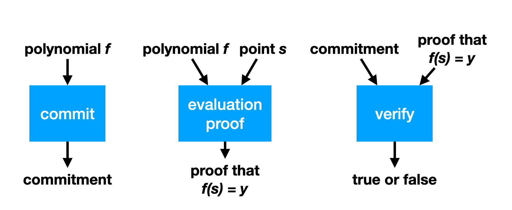
Polynomial commitments

To construct SNARKs we use polynomial commitments. A polynomial commitment scheme for a field $F$ (or it could even be a ring) is a way of committing to a polynomial $f \in F [x]$ to get a commitment $c$ , in such a way that for any $α \in F$ , you can provide $y = f (α)$ , along with an “opening proof” $π$ that proves that the polynomial committed to in $c$ equals $y$ when evaluated at $α$ .

In other words, it is a type of commitment $C$ , a type of randomness $R$ , a type of opening proof $P$ along with algorithms

$commit : F [x] \times R \to C open : C \times F \times (F [x] \times R) \to F \times P verify : C \times (F \times P) \to Bool$

such that for any $f \in F [x], r \in R, α \in F$ , we have

$c := commit (f, r) verify (c, open (c, α, (f, r))) = true$

and if $b \neq = f (α)$ then it is not possible to compute $π \in P$ such that

$verify (c, (b, π)) = true$

In other words, if $b \neq = f (α)$ then every $π$ which is feasible to compute results in $verify (c, (b, π)) = false$ .

One thing that’s pretty cool is that because polynomial commitment schemes let you construct zk-SNARKs, polynomial commitment schemes imply commitment schemes with arbitrary opening functionality. TODO

Constructing polynomial commitment schemes

All known constructions of polynomial commitment schemes are a bit complicated. The easiest to describe is called the Kate (pronounced “kah-TAY”) scheme, also known as “KZG”. It requires a “prime-order group with a pairing”, which is three groups $G_{1}, G_{2}, G_{T}$ of prime order $p$ (hence, all isomorphic cyclic groups) together with a function $e : G_{1} \times G_{2} \to G_{T}$ such that for any $a_{1}, a_{2} \in Z$ , $g_{1} \in G_{1}$ , $g_{2} \in G_{2}$ , we have

$e (a_{1} \cdot g_{1}, a_{2} \cdot g_{2}) = a_{1} a_{2} \cdot e (g_{1}, g_{2})$

$e$ is called a “pairing” or a “bilinear pairing”. What this lets us do is “multiply in the scalar” but only once.

Fix a degree bound $d$ on the polynomials we would like to be able to commit to. The KZG scheme, will let us commit to polynomials in $F_{p} [x]_{< d}$ . As a preliminary, fix generators $g_{1} \in G_{1}, g_{2} \in G_{2}$ arbitrarily.

The first thing to know about the KZG scheme is it requires that we randomly sample some group elements to help us. This is the dreaded and much discussed trusted setup. So, anyway, we start by sampling $τ$ at random from $F_{p}$ and computing for $i < d$ ,

$h_{i} := (τ^{i}) \cdot g_{1} w := τ \cdot g_{2}$

And then throw away $τ$ . The security depends on no one knowing $τ$ , which is sometimes referred to as the toxic waste of the trusted setup. Basically we compute the generator scaled by powers of $τ$ up to the degree bound. We make a security assumption about the groups which says that all anyone can really do with group elements is take linear combinations of them.

Now suppose we have a polynomial $f \in F_{p} [x]_{< d}$ with $f = \sum_{i < d} a_{i} x^{i}$ that we would like to commit to. We will describe a version of the scheme that is binding but not hiding, so it may leak information about the polynomial. Now, to commit to $f$ , we compute

$c_{f} := commit (f) = a_{0} \cdot h_{0} + a_{1} \cdot h_{1} + \dots + a_{d - 1} \cdot h_{d - 1}$

so that $c_{f} \in G_{1}$ and

$c_{f} = i < d \sum a_{i} \cdot h_{i} = i < d \sum a_{i} \cdot τ^{i} g_{1} = i < d \sum (a_{i} τ^{i}) \cdot g_{1} = (i < d \sum a_{i} τ^{i}) \cdot g_{1} = f (τ) \cdot g_{1}$

So $c_{f}$ is $g_{1}$ scaled by $f (τ)$ and the fact that $G_{1}$ is an $F_{p}$ -module (i.e. a vector space whose scalars come from $F_{p}$ ) means we can compute $f (τ) \cdot g_{1}$ from the $h_{i}$ and the coefficients of $f$ without knowing $τ$ .

Now how does opening work? Well, say we want to open at a point $a$ to $b = f (a)$ . Then the polynomial $f - b$ vanishes at $a$ , which means that it is divisible by the polynomial $x - a$ (exercise, use polynomial division and analyze the remainder).

So, the opener can compute the polynomial

$q := \frac{f - b}{x - a}$

and commit to it as above to get a commitment $c_{q}$ . And $c_{q}$ will be the opening proof. It remains only to describe verification. It works like this

$verify (c_{f}, (b, c_{q})) := e (c_{q}, w - a \cdot g_{2}) =_{?} e (c_{f} - b \cdot g_{1}, g_{2})$

This amounts to checking: “is the polynomial committed to $c_{f}$ equal to the polynomial committed to by $c_{q}$ times $x - a$ ”?

To see why, remember that $w = τ \cdot g_{2}$ , and say $c_{q} = s_{q} \cdot g_{1}$ and $c_{f} = s_{f} \cdot g_{1}$ so we are checking

$e (s_{q} \cdot g_{1}, (τ - a) \cdot g_{2}) =_{?} e ((s_{f} - b) \cdot g_{1}, g_{2})$

which by the bilinearity of the pairing is the same as checking

$s_{q} \cdot (τ - a) = s_{f} - b$

Bootleproof inner product argument

Polynomial commitments

A polynomial commitment is a scheme that allows you to commit to a polynomial (i.e. to its coefficients). Later, someone can ask you to evaluate the polynomial at some point and give them the result, which you can do as well as provide a proof of correct evaluation.

Schwartz-Zippel lemma

TODO: move this section where most relevant

Let $f (x)$ be a non-zero polynomial of degree $d$ over a field $F$ of size $n$ , then the probability that $f (s) = 0$ for a randomly chosen $s$ is at most $\frac{d}{n}$ .

In a similar fashion, two distinct degree $d$ polynomials $g (X)$ and $h (X)$ can at most intersect in $d$ points. This means that the probability that $g (s) = h (s)$ on a random $s \leftarrow F$ is $\frac{d}{∣ F ∣}$ . This is a direct corollary of the Schwartz-Zipple lemma, because it is equivalent to the probability that $f (s) = 0$ with $f (X) = g (X) - h (X)$

Inner product argument

What is an inner product argument?

The inner product argument is the following construction: given the commitments (for now let’s say the hash) of two vectors $a$ and $b$ of size $n$ and with entries in some field $F$ , prove that their inner product $⟨ a, b ⟩$ is equal to $z$ .

There exist different variants of this inner product argument. In some versions, none of the values ( $a$ , $b$ and $z$ ) are given, only commitments. In some other version, which is interesting to us and that I will explain here, only $a$ is unknown.

How is that useful?

Inner products arguments are useful for several things, but what we’re using them for in Mina is polynomial commitments. The rest of this post won’t make too much sense if you don’t know what a polynomial commitment is, but briefly: it allows you to commit to a polynomial $f$ and then later prove its evaluation at some point $s$ . Check my post on Kate polynomial commitments for more on polynomial commitment schemes.

How does that translate to the inner product argument though? First, let’s see our polynomial $f$ as a vector of coefficients:

$f = (f_{0}, \dots, f_{n}) such that f (x) = f_{0} + f_{1} x + f_{2} x^{2} + \dots + f_{n} x^{n}$

Then notice that

$f (s) = ⟨ f, (1, s, s^{2}, \dots, s^{n})⟩$

And here’s our inner product again.

The idea behind Bootleproof-type of inner product argument

The inner product argument protocol I’m about to explain was invented by Bootle et al. It was later optimized in the Bulletproof paper (hence why we unofficially call the first paper bootleproof), and then some more in the Halo paper. It’s the later optimization that I’ll explain here.

A naive approach

So before I get into the weeds, what’s the high-level? Well first, what’s a naive way to prove that we know the pre-image of a hash $h$ , the vector $a$ , such that $⟨ a, b ⟩ = z$ ? We could just reveal $a$ and let anyone verify that indeed, hashing it gives out $h$ , and that it also verifies the equation $⟨ a, b ⟩ = z$ .

$⟨ a, b ⟩ = z given b, z, and a hash of a open proof a$

Obliviously, we have to reveal $a$ itself, which is not great. But we’ll deal with that later, trust me. What we want to tackle first here is the proof size, which is the size of the vector $a$ . Can we do better?

Reducing the problem to a smaller problem to prove

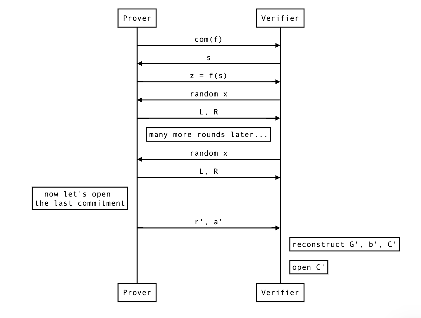
The inner product argument reduces the opening proof by using an intermediate reduction proof:

$⟨ a, b ⟩ = z given b, z, and a hash of a reduction proof ⟨ a^{'}, b^{'} ⟩ = z^{'} given b^{'}, z^{'}, and a hash of a^{'} open proof a^{'}$

Where the size of $a^{'}$ is half the size of $a$ , and as such the final opening proof ( $a^{'}$ ) is half the size of our naive approach.

The reduction proof is where most of the magic happens, and this reduction can be applied many times ( $l o g_{2} (n)$ times to be exact) to get a final opening proof of size 1. Of course the entire proof is not just the final opening proof of size 1, but all the elements involved in the reduction proofs. It can still be much smaller than the original proof of size $n$ .

So most of the proof size comes from the multiple reduction subproofs that you’ll end up creating on the way. Our proof is really a collection of miniproofs or subproofs.

One last thing before we get started: Pedersen hashing and commitments

To understand the protocol, you need to understand commitments. I’ve used hashing so far, but hashing with a hash function like SHA-3 is not great as it has no convenient mathematical structure. We need algebraic commitments, which will allow us to prove things on the committed value without revealing the value committed. Usually what we want is some homomorphic property that will allow us to either add commitments together or/and multiply them together.

For now, let’s see a simple non-hiding commitment: a Pedersen hash. To commit to a single value $x$ simply compute:

$x G$

where the discrete logarithm of $G$ is unknown. To open the commitment, simply reveal the value $x$ .

We can also perform multi-commitments with Pedersen hashing. For a vector of values $(x_{1}, \dots, x_{k})$ , compute:

$x_{1} G_{1} + \dots + x_{k} G_{k}$

where each $G_{i}$ is distinct and has an unknown discrete logarithm as well. I’ll often shorten the last formula as the inner product $⟨ x, G ⟩$ for $x = (x_{1}, \dots, x_{k})$ and $G = (G_{1}, \dots, G_{k})$ . To reveal a commitment, simply reveal the values $x_{i}$ .

Pedersen hashing allow commitents that are non-hiding, but binding, as you can’t open them to a different value than the originally committed one. And as you can see, adding the commitment of $x$ and $y$ gives us the commitment of $x + y$ :

$x G + y G = (x + y) G$

which will be handy in our inner product argument protocol

The protocol

Set up

Here are the settings of our protocol. Known only to the prover, is the secret vector

$a = (a_{1}, a_{2}, a_{3}, a_{4})$

The rest is known to both:

$G = (G_{1}, G_{2}, G_{3}, G_{4})$ , a basis for Pedersen hashing
$A = ⟨ a, G ⟩$ , the commitment of $a$
$b = (b_{1}, b_{2}, b_{3}, b_{4})$ , the powers of some value $s$ such that $b = (1, s, s^{2}, s^{3})$
the result of the inner product $z = ⟨ a, b ⟩$

For the sake of simplicity, let’s pretend that this is our problem, and we just want to halve the size of our secret vector $a$ before revealing it. As such, we will only perform a single round of reduction. But you can also think of this step as being already the reduction of another problem twice as large.

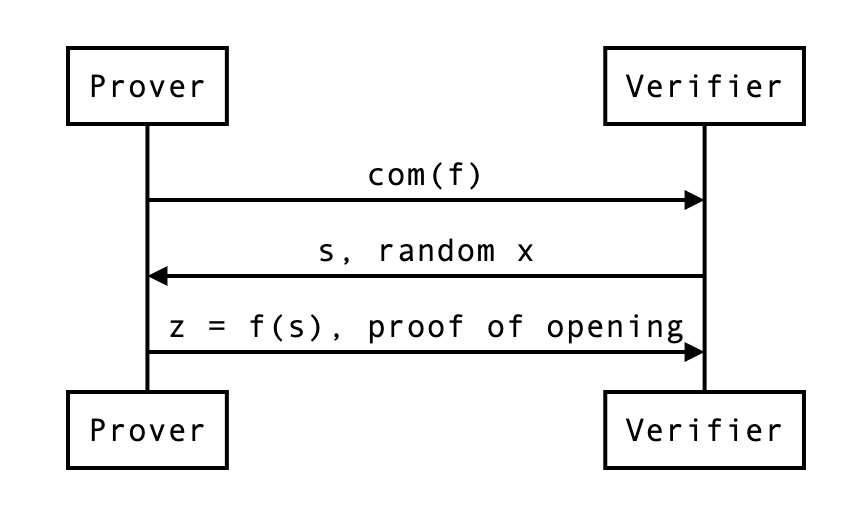
We can picture the protocol as follows:

The prover first sends a commitment to the polynomial $f$ .
The verifier sends a point $s$ , asking for the value $f (s)$ . To help the prover perform a proof of correct evaluation, they also send a random challenge $x$ . (NOTE: The verifier sends the random challenge $x$ ONLY AFTER they receive the $z = f (s)$ )
The prover sends the result of the evaluation, $z$ , as well as a proof.

inner 1

Does that make sense? Of course what’s interesting to us is the proof, and how the prover uses that random $x$ .

Reduced problem

First, the prover cuts everything in half. Then they use $x$ to construct linear combinations of these cuts:

$a^{'} = x^{- 1} (a_{1} a_{2}) + x (a_{3} a_{4})$
$b^{'} = x (b_{1} b_{2}) + x^{- 1} (b_{3} b_{4})$
$G^{'} = x (G_{1} G_{2}) + x^{- 1} (G_{3} G_{4})$

This is how the problem is reduced to $⟨ a^{'}, b^{'} ⟩ = z^{'}$ .

At this point, the prover can send $a^{'}$ , $b^{'}$ , and $z^{'}$ and the verifier can check if indeed $⟨ a^{'}, b^{'} ⟩ = z^{'}$ . But that wouldn’t make much sense would it? Here we also want:

a proof that proving that statement is the same as proving the previous statement ( $⟨ a, b ⟩ = z$ )
a way for the verifier to compute $z^{'}$ and $b^{'}$ and $A^{'}$ (the new commitment) by themselves.

The actual proof

The verifier can compute $b^{'}$ as they have everything they need to do so.

What about $A^{'}$ , the commitment of $a^{'}$ which uses the new $G^{'}$ basis. It should be the following value:

$A^{'} = = = = ⟨ a^{'}, G^{'} ⟩ (x^{- 1} a_{1} + x a_{3}) (x G_{1} + x^{- 1} G_{3}) + (x^{- 1} a_{2} + x a_{4}) (x G_{2} + x^{- 1} G_{4}) A + x^{- 2} (a_{1} G_{3} + a_{2} G_{4}) + x^{2} (a_{3} G_{1} + a_{4} G_{2}) A + x^{- 2} L_{a} + x^{2} R_{a}$

So to compute this new commitment, the verifier needs:

the previous commitment $A$ , which they already have
some powers of $x$ , which they can compute
two curve points $L_{a}$ and $R_{a}$ , which the prover will have to provide to them

What about $z^{'}$ ? Recall:

$a^{'} = (x^{- 1} a_{1} + x a_{3} x^{- 1} a_{2} + x a_{4})$
$b^{'} = (x b_{1} + x^{- 1} b_{3} x b_{2} + x^{- 1} b_{4})$

So the new inner product should be:

$z^{'} = = = = ⟨ a^{'}, b^{'} ⟩ ⟨ (x^{- 1} a_{1} + x a_{3} x^{- 1} a_{2} + x a_{4}), (x b_{1} + x^{- 1} b_{3} x b_{2} + x^{- 1} b_{4}) ⟩ (a_{1} b_{1} + a_{2} b_{2} + a_{3} b_{3} + a_{4} b_{4}) + x^{- 2} (a_{1} b_{3} + a_{2} b_{4}) + x^{2} (a_{3} b_{1} + a_{4} b_{2}) z + x^{- 2} (L_{z}) + x^{2} (R_{z})$

Similarly to $A^{'}$ , the verifier can recompute $z^{'}$ from the previous value $z$ and two scalar values $L_{z}$ and $R_{z}$ which the prover needs to provide.

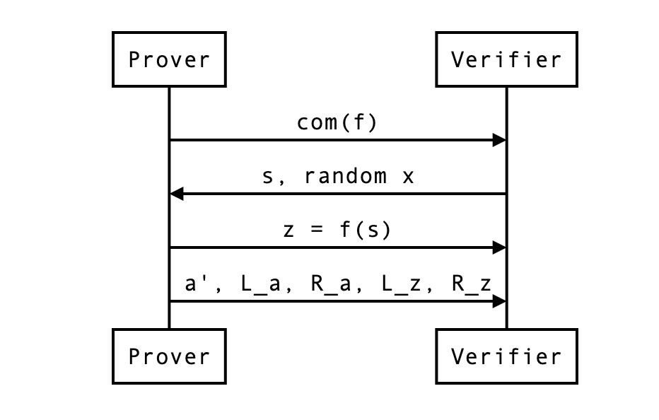
So in the end, the proof has become:

the vector $a^{'}$ which is half the size of $a$
the $L_{a}, R_{a}$ curve points (around two field elements, if compressed)
the $L_{z}, R_{z}$ scalar values

We can update our previous diagram:

inner 2

In our example, the naive proof was to reveal $a$ which was 4 field elements. We are now revealing instead 2 + 2 + 2 = 6 field elements. This is not great, but if $a$ was much larger (let’s say 128), the reduction in half would still be of 64 + 2 + 2 = 68 field elements. Not bad no? We can do better though…

The HALO optimization

The HALO optimization is similar to the bulletproof optimization, but it further reduces the size of our proof, so I’ll explain that directly.

With the HALO optimization, the prover translates the problem into the following:

$C = A + z U = ⟨ a, G ⟩ + ⟨ a, b ⟩ U$

This is simply a commitment of $a$ and $z$ .

A naive proof is to reveal $a$ and let the verifier check that it is a valid opening of the following commitment. Then, that commitment will be reduced recursively to commitments of the same form.

$C^{'} = A^{'} + z^{'} U = ⟨ a^{'}, G^{'} ⟩ + ⟨ a^{'}, b^{'} ⟩ U$

The whole point is that the reduction proofs will be smaller than our previous bootleproof-inspired protocol.

How does the reduction proof work? Notice that this is the new commitment:

$C^{'} = = ⟨ a^{'}, G^{'} ⟩ + ⟨ a^{'}, b^{'} ⟩ U [A + x^{- 2} L_{a} + x^{2} R_{a}] + [z + x^{- 2} (L_{z}) + x^{2} (R_{z})] U$

This is simply from copy/pasting the equations from the previous section. This can be further reduced to:

$C^{'} = C + x^{- 2} (L_{a} + L_{z} U) + x^{2} (R_{a} + R_{z} U)$

And now you see that the verifier now only needs, in addition to $a^{'}$ , two curve points (~ 2 field elements):

$L = L_{a} + L_{z} U$
$R = R_{a} + R_{z} U$

this is in contrast to the 4 field elements per reduction needed without this optimization. Much better right?

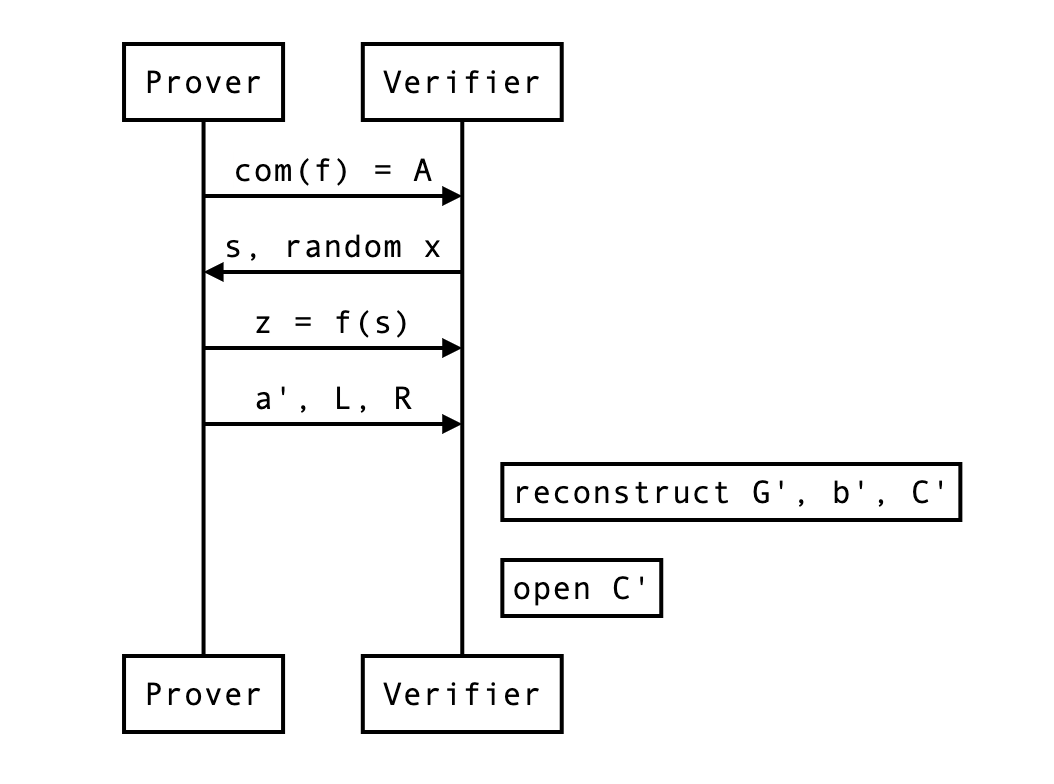
At the end of a round (or the protocol) the verifier can compute the expected commitment $C^{'}$ as such:

$C^{'} = C + x^{- 2} L + x^{2} R$

and open it by computing the following and checking it is indeed equal to $C^{'}$ :

$⟨ a^{'}, G^{'} ⟩ + ⟨ a^{'}, b^{'} ⟩ U$

For this, the verifier needs to recompute $G^{'}$ and $b^{'}$ by themselves, which they can as they have all the necessary information. We can update our previous diagram:

inner 3

What about zero-knowledge?

Didn’t we forget something? Oh right, we’re sending $a^{'}$ in clear, a single element that will leak some information about the original vector $a$ (as it is a linear combination of that original vector).

The simple solution is to alter our pedersen commitment to make it hiding on top of being binding:

$C = A + z U + rH = ⟨ a, G ⟩ + ⟨ a, b ⟩ U + rH$

where H is another generator we don’t know the discrete logarithm of, and $r$ is a random scalar value generated by the prover to blind the commitment.

But wait, each $L$ and $R$ also leaks some! As they are also made from the original secret vector $a$ . Remember, $L = L_{a} + L_{z} U$ No worries, we can perform the same treatment on that curve point and blind it like so:

$L = L_{a} + L_{z} U + r_{L} H$
$R = R_{a} + R_{z} U + r_{R} H$

In order to open the final commitment, the verifier first recomputes the expected commitment as before:

$C^{'} = C + x^{- 2} L + x^{2} R$

then use $a^{'}$ and the final blinding value $r^{'}$ sent by the prover (and composed of $r$ and all the rounds’ $r_{L}$ and $r_{R}$ ), as well as reconstructed $G^{'}$ and $b^{'}$ to open the commitment:

$⟨ a^{'}, G^{'} ⟩ + ⟨ a^{'}, b^{'} ⟩ U + r^{'} H$

with $r^{'}$ being equal to something like $r + \sum_{i} (r_{L i} + r_{R i})$

At this point, the protocol requires the sender to send:

2 curve points $L$ and $R$ per rounds
1 scalar value $a^{'}$ for the final opening
1 blinding (scalar) value $r^{'}$ for the final opening

But wait… one last thing. In this protocol the prover is revealing $a^{'}$ , and even if they were not, by revealing $r^{'}$ they might allow someone to recompute $a^{'}$ … The HALO paper contains a generalized Schnorr protocol to open the commitment without revealing $a^{'}$ nor $r^{'}$ .

from Vanishree:

So in general the more data we send the more randomness we need to ensure the private aspects are hidden, right
The randomness in a commitment is because we are sending the commitment elements
The random elements mixed with the polynomial (in the new zkpm technique) is because we send evaluations of the polynomial at zeta and zeta omega later
Zk in Schnorr opening is because we reveal the opening values

where can I find a proof? perhaps appendix C of https://eprint.iacr.org/2017/1066.pdf

The real protocol, and a note on non-interactivity

Finally, we can look at what the real protocol end up looking at with $l o g_{2} (n)$ rounds of reduction followed by a commitment opening.

inner 4

So far the protocol was interactive, but you can make it non-interactive by simply using the Fiat-Shamir transformation. That’s all I’ll say about that.

Different functionalities

There’s a number of useful stuff that we can do on top of a bootleproof-style polynomial commitment. I’ll briefly list them here.

Enforcing an upperbound on the polynomial degree

Imagine that you want to enforce a maximum degree on a committed polynomial. You can do that by asking the prover to shift the coefficients of the polynomial to the right, so much that it becomes impossible to fit them if the polynomial were to be more than the maximum degree we wanted to enforce. This is equivalent to the following:

$right_shift (f) = x^{n - ma x} f$

When the verifier verifies the opening, they will have to right shift the received evaluation in the same way.

$right_shift (f (z)) = z^{n - ma x} f (z)$

Aggregating opening proofs for several polynomials

Insight:

$⟨ f + v \cdot g, x ⟩ = f (x) + v \cdot g (x)$

Aggregating opening proofs for several evaluations

Insight:

$⟨ f, x_{1} + u \cdot x_{2} ⟩ = f (x_{1}) + u \cdot f (x_{2})$

Double aggregation

Insight:

$⟨ f + v \cdot g, x_{1} + u \cdot x_{2} ⟩ = f (x_{1}) + v \cdot g (x_{1}) + u \cdot (f (x_{2}) + v \cdot g (x_{2}))$

Note that this kind of aggregation forces us to provide all combinations of evaluations, some of which might not be needed (for example, $f (x_{2})$ ).

Splitting a polynomial

If a polynomial is too large to fit in one SRS, you can split it in chuncks of size at most $n$

Proof of correct commitment to a polynomial

That is useful in HALO. Problem statement: given a commitment $A$ , and a polynomial $f$ , prove to me that the $A = co m (f)$ . The proof is simple:

generate a random point $s$
evaluate $f$ at $s$ , $f (s) = y$
ask for an evaluation proof of $A$ on $s$ . If it evaluates to $y$ as well then $A$ is a commitment to $f$ with overwhelming probability

Two Party Computation

This section introduces cryptographic primitives and optimizations of two-party computation protocols based on Garbled Circuit (GC) and Oblivious Transfer (OT).

More specifically, this section will cover the following contents.

Garbled Circuit
- Including the Free-XOR, Point-and-Permute, Row-Reduction and Half-Gate optimizations.
Oblivious Transfer
- Including base OT and OT extension. Note that we focus on maliciously secure OT protocols. The overhead is comparable to protocols with semi-honest security.
Two-Party Computation Protocol
- This is the well-known Yao’s 2PC protocol based on GC and OT.

Garbled Circuits

For general-purpose secure computation protocols, we often view functions as arithmetic circuits or boolean circuits. We consider boolean circuits because our applications involve in securely computing ciphers (e.g., AES), which consist of massive boolean gates.

Boolean Circuits

Boolean circuits consists of $AND$ gates ( $a AND b = a \land b$ ) and $XOR$ gates ( $a XOR b = a \oplus b$ ). These two gates are universal and we could represent any polynomial-size functions with them. In 2PC protocols, we also use $INV$ gates ( $INV (a) = 1 \oplus a$ ) for optimization.

According to the Free-XOR optimization (see the next subsection), the $XOR$ gates and $INV$ gates are free, then one prefers to represent a function with more $XOR$ and $INV$ gates, while less $AND$ gates.

For some commonly used functions (e.g., AES, SHA256), one usually uses hand-optimized circuits for efficiency, and stores them in files. The most popular circuit representation is the Bristol Fashion, which is also used in zkOracles.

The following Bristol fashion circuit is part of AES-128.

36663 36919
2 128 128 
1 128 

2 1 128 0 33254 XOR
2 1 129 1 33255 XOR
2 1 130 2 33256 XOR
2 1 131 3 33257 XOR
2 1 132 4 33258 XOR
2 1 133 5 33259 XOR
2 1 134 6 33260 XOR
...
2 1 3542 3546 3535 AND
2 1 3535 3459 3462 XOR
2 1 3543 3541 3534 AND
...
1 1 3452 3449 INV
...

The first line

36663 36919

means that the entire circuit has 36663 gates and 36919 wires.

The second line

2 128 128

means that the circuit has 2 inputs, both inputs have 128 bits.

The third line

1 128

means that the circuit has 1 output, and the length is 128 bits.

The following lines are the gates in the circuit. For example

2 1 128 0 33254 XOR

means that this gate has a fan-in of 2 and fan-out of 1. The first input wire is 128 (the number of wires), the second input wire is 0, and the output wire is 33254. The operation of this gate is $XOR$ .

2 1 3542 3546 3535 AND

means that this gate has a fan-in of 2 and fan-out of 1. The first input wire is 3542, the second input wire is 3546, and the output wire is 3535. The operation of this gate is $AND$ .

1 1 3452 3449 INV

means that this gate has a fan-in of 1 and fan-out of 1. The input wire is 3452, and the output wire is 3449. The operation of this gate is $INV$

Basics

Garbled circuit is a core building block of two-party computation. The invention of garbled circuit was credited to Andrew Yao, with plenty of optimizations the state-of-the-art protocols are extremely efficient. This subsection will first introduce the basic idea of garbled circuit.

Garbled circuit involves two parties: the garbler and the evaluator. The garbler takes as input the circuit and the inputs, generates the garbled circuit and encoded inputs. The evaluator takes as input the garbled circuit and encoded inputs, evaluates the garbled circuit and decodes the result into outputs.

The security of garbled circuit ensures that the evaluator only gets the outputs without any additional information.

Given a circuit and related inputs, the garbler handles the circuit as follows.

For each gate in the circuit $C$ , the garbler writes down the truth table of this gate. Taking an $AND$ gate for example. The truth table is as follows. Note that for different $AND$ gates, the wires $a, b, c$ may be different.

$a$	$b$	$c$
$0$	$0$	$0$
$0$	$1$	$0$
$1$	$0$	$0$
$1$	$1$	$1$

The garbler chooses two uniformly random $128$ -bit strings for each wire. We call these strings the truth labels. Label $0$ represents the value $0$ and label $1$ represents the value $1$ . The garbler replaces the truth table with the following label table.

$a$	$b$	$c$
$X_{a}^{0}$	$X_{b}^{0}$	$X_{c}^{0}$
$X_{a}^{0}$	$X_{b}^{1}$	$X_{c}^{0}$
$X_{a}^{1}$	$X_{b}^{0}$	$X_{c}^{0}$
$X_{a}^{1}$	$X_{b}^{1}$	$X_{c}^{1}$

The garbler turns this label table into a garbled gate by encrypting the $c$ labels using a symmetric double-key cipher with $a, b$ labels as the keys. The garbler randomly permutes the ciphertexts to break the relation between the label and value.

Garbled Gate
$Enc_{X_{a}^{0}, X_{b}^{0}} (X_{c}^{0})$
$Enc_{X_{a}^{0}, X_{b}^{1}} (X_{c}^{0})$
$Enc_{X_{a}^{1}, X_{b}^{0}} (X_{c}^{0})$
$Enc_{X_{a}^{1}, X_{b}^{1}} (X_{c}^{1})$

The garbled circuit $G C (C)$ consists of all garbled gates according to the circuit.
Let $I = I_{0} ∥ \dots ∥ I_{k}$ be the input, where $I_{i} \in {0, 1}$ , let $w_{0}, \dots, w_{k}$ be the wires of the input. The garbler sends ${X_{w_{i}}^{I_{i}}}_{i \in [k]}$ and $G C (C)$ to the evaluator. The garbler also reveals the relation of the output labels and the truth values. For example, for each output wire, the label is chosen by setting the least significant bit to be the truth value.

Given the circuit $C$ , the garbled circuit $G C (C)$ and the encoded inputs ${X_{w_{i}}^{I_{i}}}_{i \in [k]}$ , the evaluator does the following.

Uses the encoded inputs as keys, the evaluator goes through all the garbled gates one by one and tries to decrypt all the four ciphertexts according to the circuit.
The encryption scheme is carefully designed to ensure that the evaluator could only decrypt to one valid message. For example, the $c$ label is encrypted by padding $0^{40}$ , and the decrypted message contains $0^{40}$ is considered to be valid.
After the evaluator gets all the labels of the output wires, he/she extracts the output value. For example, just take the least significant bit of the label.

Note that the above description of garbled circuit is very inefficient, the following subsections will introduce optimizations to improve it.

Point and Permute

As described in the last subsection, the evaluator has to decrypt all the four ciphertexts of all the garbled gates, and extracts the valid label. This trial decryption results in 4 decryption operations and ciphertext expansion.

The point-and-permute optimization of garbled circuit in BMR90 only needs 1 decryption and no ciphertext expansion. It works as follows.

For the two random labels of each wire, the garbler assigns uniformly random color bits to them. For example for the wire $a$ , the garbler chooses uniformly random labels $X_{a}^{0}, X_{a}^{1}$ , and then sets $LSB (X_{a}^{1}) = 1 \oplus LSB (X_{a}^{0})$ . Note that the random color bits are independent of the truth bits.
Then the garbled gate becomes the following. Suppose the relation of the labels and color bits are $(X_{a}^{0}, X_{a}^{1}) \leftrightarrow (0, 1)$ , $(X_{b}^{0}, X_{b}^{1}) \leftrightarrow (1, 0)$ , $(X_{c}^{0}, X_{c}^{1}) \leftrightarrow (0, 1)$

Color Bits $(a, b, c)$	Garbled Gate
$(0, 1, 0)$	$Enc_{X_{a}^{0}, X_{b}^{0}} (X_{c}^{0})$
$(0, 0, 0)$	$Enc_{X_{a}^{0}, X_{b}^{1}} (X_{c}^{0})$
$(1, 1, 0)$	$Enc_{X_{a}^{1}, X_{b}^{0}} (X_{c}^{0})$
$(1, 0, 1)$	$Enc_{X_{a}^{1}, X_{b}^{1}} (X_{c}^{1})$

Reorder the 4 ciphertexts canonically by the color bits of the input labels as follows.

Color Bits $(a, b, c)$	Garbled Gate
$(0, 0, 0)$	$Enc_{X_{a}^{0}, X_{b}^{1}} (X_{c}^{0})$
$(0, 1, 0)$	$Enc_{X_{a}^{0}, X_{b}^{0}} (X_{c}^{0})$
$(1, 0, 1)$	$Enc_{X_{a}^{1}, X_{b}^{1}} (X_{c}^{1})$
$(1, 1, 0)$	$Enc_{X_{a}^{1}, X_{b}^{0}} (X_{c}^{0})$

When the evaluator gets the input label, say $X_{a}^{1}, X_{b}^{1}$ , the evaluator first extracts the color bits $(LSB (X_{a}^{1}), LSB (X_{b}^{1})) = (1, 0)$ and decrypts the corresponding ciphertext (the third one in the above example) to get a output label.

Encryption Instantiation

The encryption algorithm is instantiated with hash function (modeled as random oracle) and one-time pad. The hash function could be truncated $SHA 256$ . The garbled gate is then as follows.

Color Bits $(a, b, c)$	Garbled Gate
$(0, 0, 0)$	$H (X_{a}^{0}, X_{b}^{1}) \oplus X_{c}^{0}$
$(0, 1, 0)$	$H (X_{a}^{0}, X_{b}^{0}) \oplus X_{c}^{0}$
$(1, 0, 1)$	$H (X_{a}^{1}, X_{b}^{1}) \oplus X_{c}^{1}$
$(1, 1, 0)$	$H (X_{a}^{1}, X_{b}^{0}) \oplus X_{c}^{0}$

For security and efficiency reasons, one usually uses tweakable hash functions: $H (tweak, \cdot)$ , where $tweak$ is public and unique for different groups of calls to $H$ . E.g., $tweak$ could be the gate identifier. Then the garbled gate is as follows. The optimization of tweakable hash functions is given in following subsections.

Color Bits $(a, b, c)$	Garbled Gate
$(0, 0, 0)$	$H (gid, X_{a}^{0}, X_{b}^{1}) \oplus X_{c}^{0}$
$(0, 1, 0)$	$H (gid, X_{a}^{0}, X_{b}^{0}) \oplus X_{c}^{0}$
$(1, 0, 1)$	$H (gid, X_{a}^{1}, X_{b}^{1}) \oplus X_{c}^{1}$
$(1, 1, 0)$	$H (gid, X_{a}^{1}, X_{b}^{0}) \oplus X_{c}^{0}$

Free XOR

The Free-XOR optimization significantly improves the efficiency of garbled circuit. The garbler and evaluator could handle $XOR$ gates for free! The method is given in KS08.

The garbler chooses a global uniformly random string $Δ$ with $LSB (Δ) = 1$ .
For any $XOR$ gate with input wires $a, b$ and output wire $c$ , the garbler chooses uniformly random labels $X_{a}$ and $X_{b}$ .
Let $X_{a}$ and $X_{a} \oplus Δ$ denote the 0 label and 1 label for input wire $a$ , respectively. Similarly for wire $b$ .
Let $X_{a} \oplus X_{b}$ and $X_{a} \oplus X_{b} \oplus Δ$ denote the 0 label and 1 label for input wire $c$ , respectively.
The garbler does not need to send garbled gate for each $XOR$ gate. The evaluator locally $XOR$ s the input labels of $XOR$ gate to gets the output label. This is correct because given a $XOR$ gate, the label table could be as follows.

$a$	$b$	$c$
$X_{a}$	$X_{b}$	$X_{a} \oplus X_{b}$
$X_{a}$	$X_{b} \oplus Δ$	$X_{a} \oplus X_{b} \oplus Δ$
$X_{a} \oplus Δ$	$X_{b}$	$X_{a} \oplus X_{b} \oplus Δ$
$X_{a} \oplus Δ$	$X_{b} \oplus Δ$	$X_{a} \oplus X_{b}$

Here are some remarks of the Free-XOR optimization.

Free XOR is compatible with the point-and-permute optimization because $LSB (Δ) = 1$ .
The garbler should keep $Δ$ private all the time for security reasons.
Garbling $AND$ gate is the same as before except that all the labels are of the form $(X, X \oplus Δ)$ for uniformly random $X$ .

Row Reduction

With the Free-XOR optimization, the bottleneck of garbled circuit is to handle $AND$ gates. Row reduction aims to reduce the number of ciphertexts of each garbled $AND$ gate. More specifically, it reduces $4$ ciphertexts into $3$ . The optimization is given in the NPS99 paper.

To be compatible with the Free-XOR optimization, the garbled $AND$ gates are of the following form (still use the example in the point-and-permute optimization).

Color Bits $(a, b, c)$	Garbled Gate
$(0, 0, 0)$	$H (X_{a}, X_{b} \oplus Δ) \oplus X_{c}$
$(0, 1, 0)$	$H (X_{a}, X_{b}) \oplus X_{c}$
$(1, 0, 1)$	$H (X_{a} \oplus Δ, X_{b} \oplus Δ) \oplus X_{c} \oplus Δ$
$(1, 1, 0)$	$H (X_{a} \oplus Δ, X_{b}) \oplus X_{c}$

Since $H$ is modeled as a random oracle, one could set the first row of the above garbled gate as $0$ , and then we could remove that row from the garbled gate. This means that we could choose $X_{c} = H (X_{a}, X_{b} \oplus Δ)$ . Therefore, the garbled circuit is changed as follows.

Color Bits $(a, b, c)$	Garbled Gate
$(0, 1, 0)$	$H (X_{a}, X_{b}) \oplus H (X_{a}, X_{b} \oplus Δ)$
$(1, 0, 1)$	$H (X_{a} \oplus Δ, X_{b} \oplus Δ) \oplus H (X_{a}, X_{b} \oplus Δ) \oplus Δ$
$(1, 1, 0)$	$H (X_{a} \oplus Δ, X_{b}) \oplus H (X_{a}, X_{b} \oplus Δ)$

The evaluator handles garbled $AND$ gates as before, except he/she directly computes the hash function if the color bits are $(0, 0)$

Half Gate

The Half-Gate optimization further reduces the number of ciphertexts from $3$ to $2$ . This is also the protocol used in zkOracles, and more details of this algorithm will be given in this subsection. The algorithm is presented in the ZRE15 paper.

We first describe the basic idea behind half-gate garbling. Let’s say we want to compute the gate $a \land b = c$ . With the Free-XOR optimization, let $(X_{a}, X_{a} \oplus Δ)$ and $(X_{b}, X_{b} \oplus Δ)$ denote the input wire labels to this gate, and $(X_{c}, X_{c} \oplus Δ)$ denote the output wire labels, with $X_{a}, X_{b}, X_{c}$ each encoding $0$ .

Half-gate garbling contains two case: when the garbler knows one of the inputs, and when the evaluator knows one of the inputs.

Garbler half-gate. Considering the case of an $AND$ gate $a \land b = c$ , where $a, b$ are intermediate wires in the circuit and the garbler somehow knows in advance what the value $a$ will be.

When $a = 0$ , the garbler will garble a unary gate that always outputs $0$ . The label table is as follows.

$b$	$c$
$X_{b}$	$X_{c}$
$X_{b} \oplus Δ$	$X_{c}$

Then the garbler generates two ciphertexts: $H (X_{b}) \oplus X_{c}$ $H (X_{b} \oplus Δ) \oplus X_{c}$

When $a = 1$ , the garbler will garble a unary identity gate. The label table is as follows.

$b$	$c$
$X_{b}$	$X_{c}$
$X_{b} \oplus Δ$	$X_{c} \oplus Δ$

Then the garbler generates two ciphertexts:

$H (X_{b}) \oplus X_{c}$ $H (X_{b} \oplus Δ) \oplus X_{c} \oplus Δ$

Since $a$ is known to the garbler, the two cases shown above could be unified as follows:

$H (X_{b}) \oplus X_{c}$ $H (X_{b} \oplus Δ) \oplus X_{c} \oplus a \cdot Δ$

These two ciphertexts are then suitably permuted according to the color bits of $X_{b}$ . The evaluator takes a hash of its wire label for $X_{b}$ and decrypts the appropriate ciphertext. If $a = 0$ , he/she obtains output wire label $X_{c}$ in both values of $b$ . If $a = 1$ the evaluator obtains either $X_{c}$ or $X_{c} \oplus Δ$ , depending on the bit $b$ . Intuitively, the evaluator will never know both $X_{b}$ and $X_{b} \oplus Δ$ , hence the other ciphertext appears completely random.

By applying the row-reduction optimization, we reduce the number of ciphertexts from $2$ to $1$ as follows. $H (X_{b} \oplus Δ) \oplus H (X_{b}) \oplus a \cdot Δ$

Evaluator half-gate. Considering the case of an $AND$ gate $a \land b = c$ , where $a, b$ are intermediate wires in the circuit and the evaluator somehow knows the value $a$ at the time of evaluation. The evaluator can behave differently based on the value of $a$ .

When $a = 0$ , the evaluator should always obtain output wire label $X_{c}$ , then the garbled circuit should contains the ciphertext: $H (X_{a}) \oplus X_{c}$

When $a = 1$ , it is enough for the evaluator to obtain $R = X_{c} \oplus X_{b}$ . He/she can then $XOR$ $R$ with the other wire label (either $X_{b}$ or $X_{b} \oplus Δ$ ) to obtain either $X_{c}$ or $X_{c} \oplus Δ$ . Hence the garbler should provide the ciphertext: $H (X_{a} \oplus Δ) \oplus X_{c} \oplus X_{b}$

Combining the above two case together, the garbler should provide two ciphertexts: $H (X_{a}) \oplus X_{c}$ $H (X_{a} \oplus Δ) \oplus X_{c} \oplus X_{b}$

Note that these two ciphertext do NOT have to be permuted according to the color bit of $X_{a}$ , because the evaluator already knows $a$ . If $a = 0$ , the evaluator uses the wire label $X_{a}$ to decrypt the first ciphertext. If $a = 1$ , the evaluator uses the wire label $X_{a} \oplus Δ$ to decrypt the second ciphertext and $XOR$ s the result with the wire label for $b$ .

By applying the row-reduction optimization, we reduce the number of ciphertexts from $2$ to $1$ as follows. $H (X_{a} \oplus Δ) \oplus H (X_{a}) \oplus X_{b}$

Two halves make a whole. Considering the case to garble an $AND$ gate $a \land b = c$ , where both inputs are secret. Consider: $c = a \land b = a \land (r \oplus r \oplus b) = (a \land r) \oplus (a \land (r \oplus b))$

Suppose the garbler chooses uniformly random bit $r$ . In this case, the first $AND$ gate $(a \land r)$ can be garbled with a garbler-half-gate. If we further arrange for the evaluator to learn the value $r \oplus b$ , then the second $AND$ gate $(a \land (r \oplus b))$ can be garbled with an evaluator-half-gate. Leaking this extra bit $r \oplus b$ to the evaluator is safe, as it carries no information about the sensitive value $b$ . The remaining $XOR$ gate is free and the total cost is $2$ ciphertexts.

Actually the evaluator could learn $r \oplus b$ without any overhead. The garbler choose the color bit of the 0 label $X_{b}$ on wire $b$ . Since that color bit is chosen uniformly, it is secure to use it. Then when a particular value $b$ is on that wire, the evaluator will hold a wire label whose color bit is $b \oplus r$ .

Let $X_{b}^{0}, X_{b}^{1} = X_{b}^{0} \oplus Δ$ be the labels for $b$ , let $p = LSB (X_{b}^{0})$ . $p$ is the color bit of the wire, is a secret known only to the garbler. When the evaluator holds a wire label for $b$ whose color bit is $s$ , the label is $X_{b}^{s \oplus p}$ , corresponding to truth value $s \oplus p$ .

Full Description

Garbling. The garbling algorithm $Garble (C)$ is described as follows.

Let $CircuitInputs (C)$ , $CircuitOutputs (C)$ be the set of input and output wires of $C$ , respectively. Given a non-input wire $i$ , let $(a, b) \leftarrow InputWires (C, i)$ denote the two input wires $a, b$ of $i$ associated to an $AND$ or $XOR$ gate. Let $a \leftarrow InputsWires (C, i)$ denote the input wire $a$ of $i$ associated to an $INV$ gate. The garbler maintains three sets $E$ , $D$ and $T$ . The garbler also maintains a $counter$ initiated as $0$ .
Choose a secret global 128-bit string $Δ$ uniformly, and set $LSB (Δ) = 1$ . Let $P = X \oplus Δ$ be the label of public bit $1$ , where $X$ is chosen uniformly at random. Note that $P$ will be sent to the evaluator.
For $i \in CircuitInputs (C)$ , do the following.
- Choose $128$ -bit $X_{i}^{0}$ uniformly at random, and set $X_{i}^{1} = X_{i}^{0} \oplus Δ$ .
- Let $e_{i} = X_{i}^{0}$ and insert it to $E$ .
For any non-input wire $i$ , do the following.
- If the gate associated to $i$ is a $XOR$ gate.
  - Let $(a, b) \leftarrow GateInputs (C, i)$ .
  - Compute $X_{i}^{0} = X_{a}^{0} \oplus X_{b}^{0}$ and $X_{i}^{1} = X_{i}^{0} \oplus Δ$ .
- If the gate associated to $i$ is an $INV$ gate.
  - Let $a \leftarrow GateInputs (C, i)$ ,
  - Compute $X_{i}^{0} = X_{a}^{0} \oplus P$ and $X_{i}^{1} = X_{i}^{0} \oplus Δ$ .
- If the gate associated to $i$ is an $AND$ gate.
  - let $(a, b) \leftarrow GateInputs (C, i)$ ,
  - Let $p_{a} = LSB (X_{a}^{0})$ , $p_{b} = LSB (X_{b}^{0})$ .
  - Compute the first half gate:
  - Let $T_{G} = H (counter, X_{a}^{0}) \oplus H (counter, X_{a}^{1}) \oplus (p_{b} \cdot Δ)$ .
  - Let $X_{G}^{0} = H (counter, X_{a}^{0}) \oplus (p_{a} \cdot T_{G})$ .
  - $counter = counter + 1$ .
  - Compute the second half gate:
  - Let $T_{E} = H (counter, X_{b}^{0}) \oplus H (counter, X_{b}^{1}) \oplus X_{a}^{0}$ .
  - Let $X_{E}^{0} = H (counter, X_{b}^{0}) \oplus p_{b} \cdot (T_{E} \oplus X_{a}^{0})$
  - Let $X_{i}^{0} = X_{G}^{0} \oplus X_{E}^{0}$ , $X_{i}^{1} = X_{i}^{0} \oplus Δ$ and insert the garbled gate $(T_{G}, T_{E})$ to $T$ .
  - $counter = counter + 1$ .
For $i \in CircuitOutputs (C)$ , do the following.
- Compute $d_{i} = LSB (X_{i}^{0})$ .
- Insert $d_{i}$ into $D$ .
The garbler outputs $(G, E, D)$ .

Input Encoding. Given $E = (e_{1}, \dots, e_{ℓ})$ , the garbler encodes the input $(x_{1}, \dots, x_{ℓ}) \in {0, 1}^{ℓ}$ as follows.

For all $1 \leq i \leq ℓ$ , compute $X_{i} = e_{i} \oplus x_{i} Δ$
Outputs $X = (X_{1}, \dots, X_{ℓ})$ .

Evaluating. The evaluating algorithm $Eval (C)$ is described as follows.

The evaluator takes as input the garbled circuit $T$ and the encoded inputs $X$ .
The evaluator obtains the input labels $(X_{1}, \dots, X_{ℓ})$ from $X$ and initiates $counter = 0$ .
For any non-input wire $i$ , do the following.
- If the gate associated to $i$ is a $XOR$ gate.
  - Let $(a, b) \leftarrow GateInputs (C, i)$ .
  - Compute $X_{i} = X_{a} \oplus X_{b}$ .
- If the gate associated to $i$ is an $INV$ gate.
  - Let $a \leftarrow GateInputs (C, i)$ ,
  - Compute $X_{i} = X_{a} \oplus P$ .
- If the gate associated to $i$ is an $AND$ gate.
  - Let $(a, b) \leftarrow GateInputs (C, i)$ ,
  - Let $s_{a} = LSB (X_{a})$ , $s_{b} = LSB (X_{b})$ .
  - Parse $T_{i}$ as $(T_{G}, T_{E})$ .
  - Compute $X_{G} = H (counter, X_{a}) \oplus s_{a} \cdot T_{G}$ .
  - $counter = counter + 1$ .
  - Compute $X_{E} = H (counter, X_{b}) \oplus s_{b} (T_{E} \oplus X_{a})$ .
  - Let $X_{i} = X_{G} \oplus X_{E}$ .
For $i \in CircuitOutputs (C)$ , do the following.
- Let $Y_{i} = X_{i}$ .
- Outputs $Y$ , the set of $Y_{i}$ .

Output Decoding. Given $Y$ and $D$ , the evaluator decodes the labels into outputs as follows.

For any $i$ , compute $y_{i} = d_{i} \oplus LSB (Y_{i})$ .
Outputs all $y_{i}$ .

Fixed-Key-AES Hashes

Using fixed-key AES as a hash function in this context can be traced back to the work of Bellare et al. BHKR13, who considered fixed-key AES for circuit garbling. Prior to that point, most implementations of garbled circuits used a hash function such as $SHA 256$ , modelled as a random oracle. But Bellare et al. showed that using fixed-key AES can be up to $50 \times$ faster than using a cryptographic hash function due to hardware support for AES provided by modern processors.

Prior to BHKR13 CPU time was the main bottleneck for protocols based on circuit garbling; after the introduction of fixed-key cipher garbling, network throughput became the dominant factor. For this reason, fixed-key AES has been almost universally adopted in subsequent implementations of garbled circuits.

Several instantiations of hash function based on fix-key AES are proposed inspired by the work of Bellare et al. However, most of them have some security flaws as pointed out by GKWY20. [GKWY20] also proposes a provable secure instantiation satisfies the property called Tweakable Circular Correlation Robustness (TCCR). More discussions about the concrete security of fixed-key AES based hash are introduced in GKWWY20.

The TCCR hash based on fixed-key AES is defined as follows.

$H (i, x) = TCCR_Hash (i, x) = π (π (x) \oplus i) \oplus π (x),$ where $x$ is a $128$ -bit string, $i$ a public $128$ -bit $tweak$ , and $π (x) = AES (k, x)$ for any fixed-key $k$

Oblivious Transfer

Oblivious transfer (OT) protocol is an essential tool in cryptography that provides a wide range of applications in secure multi-party computation. The OT protocol has different variants such as $1$ -out-of- $2$ , $1$ -out-of- $n$ and $k$ -out-of- $n$ . Here we only focus on $1$ -out-of- $2$ .

An OT protocol involves two parties: the sender and the receiver. The sender has $2$ strings, whereas the receiver has a chosen bit. After the execution of this OT protocol, the receiver obtains one of the strings according to the chosen bit, but no information of the other string. Then sender get no information of the chosen bit.

                    Sender                               Receiver
    
                                      +----------+
                    (x_0,x_1) ------->|          |<------ b
                                      | OT Prot. |
                                      |          |-------> x_b 
                                      +----------+

Due to a result of Impagliazzo and Rudich in this paper, it is very unlikely that OT is possible without the use of public-key cryptography. However, OT can be efficiently extended. That is, starting with a small number of base OTs, one could create many more OTs with only symmetric primitives.

The seminal work of IKNP03 presented a very efficient protocol for extending OTs, requiring only black-box use of symmetric primitives and $λ$ base OTs, where $λ$ is the security parameter. This doc focuses on the family of protocols inspired by IKNP.

Base OT

We introduce the CO15 OT as the base OT.

Notation. The protocol is described over an additive group $(G, G, p, +)$ of prime order $p$ generated by $G$ . Denote $H : (G \times G) \times G \to {0, 1}^{λ}$ as a key-derivation function to extract a $λ$ -bit key from group elements.

Note that $H$ here is different from the tweakable hash function in garbled circuit.

In the CO15 protocol, the sender holds $n$ $128$ -bit strings ${(X_{i}^{0}, X_{i}^{1})}_{i \in [n]}$ and the receiver holds $n$ -bit string $b \in {0, 1}^{n}$ . The protocol is as follows.

The sender samples $y \leftarrow F_{p}$ , and computes $S = y \cdot G$ and $T = y \cdot S$ .
The sender sends $S$ to the receiver, who aborts if $S \in / G$ .
For $i \in [n]$ , the receiver samples $x_{i} \leftarrow F_{p}$ , and computes: $R_{i} = b_{i} S + x_{i} G$
The receiver sends ${R_{i}}_{i \in [n]}$ to the sender, who aborts if $R_{i} \in / G$ .
For $i \in [n]$ , the sender computes $k_{i}^{0} = H (S, R_{i}, y R_{i}), k_{i}^{1} = H (S, R_{i}, y R_{i} - T)$ and sends ${(c_{i}^{0} = k_{i}^{0} \oplus X_{i}^{0}, c_{i}^{1} = k_{i}^{1} \oplus X_{i}^{1})}_{i \in [n]}$ to the receiver.
For $i \in [n]$ , the receiver computes $k_{i} = H (S, R_{i}, x_{i} S)$ , and outputs $c_{i}^{b_{i}} \oplus k_{i}$

Correctness. The receiver always computes the hash of $x_{i} S = (x_{i} y) G$ . The sender sends the hashes of $y R_{i}$ and $y R_{i} - T$ . If $b_{i} = 0$ , $k_{i}^{0}$ is the hash of $y R_{i} = (y x_{i}) G$ , then the receive will get $X_{i}^{0}$ . if $b_{i} = 1$ , $k_{i}^{1}$ is the hash of $y R_{i} - T = y (S + x_{i} G) - T = (y x_{i}) G$ , then the receiver will get $X_{i}^{1}$ .

Security. We refer the security analysis to CO15.

OT Extension

To meet the large-scale demand of OTs, OT extensions can be used. An OT extension protocol works by running a small number of base OTs that are used as a base for obtaining many OTs via the use of cheap symmetric cryptographic operations only. This is conceptually similar to hybrid encryption.

In this subsection, we focus on the maliciously secure OT extension presented in KOS15.

To be compatible with the garbled circuit optimizations, Correlated OT (COT) is considered here. COT is a variant of OT, where the sender chooses a secret string $Δ$ and the receiver has a choice bit $b$ . After the protocol, then sender obtains two strings $X_{0} = X$ and $X_{1} = X \oplus Δ$ and the receiver obtains $X_{b}$ , where $X$ is a random string.

                    Sender                               Receiver
    
                                      +----------+
                       Delta  ------->|          |<------ b
                                      | COT Prot.|
     x_0 = x, x_1 = x + Delta <-------|          |-------> x_b 
                                      +----------+

Notation. Let $λ$ be the security parameter, we use $λ = 128$ in zkOracles. Identify $F_{2}^{λ}$ with the finite field $F_{2^{λ}}$ . Use “ $\cdot$ ” for multiplication in $F_{2^{λ}}$ and “ $⋆$ ” for the component-wise product in $F_{2}^{λ}$ . Given a matrix $A$ , denote its rows by subindices $a_{i}$ and its columns by superindices $a^{k}$ . Use $v [i]$ to denote the $i$ -th entry of $v$ .

The KOS15 OT protocol to generate $ℓ (≫ λ)$ OTs is described as follows.

Initialize
1. The receiver samples $λ$ pairs of $λ$ -bit seeds ${(k_{0}^{i}, k_{1}^{i})}_{i = 1}^{λ}$ .
2. The sender choose a uniformly random $λ$ -bit string $Δ$ .
3. The two parties calls the base OT with inputs $Δ$ and ${(k_{0}^{i}, k_{1}^{i})}_{i = 1}^{λ}$ .
  - Note that the sender acts as the receiver in the base OT, and the receiver acts as the sender in the base OT.
4. The sender obtains $k_{Δ_{i}}^{i}$ for $i \in [λ]$ .
Extend
1. The receiver takes as input the choice bits $x_{1}, \dots, x_{ℓ}$ , defines $ℓ^{'} = ℓ + λ + s$ , where $s$ is the statistic parameter, and we set $s = 40$ in zkOracles. Let $x = x_{1} ∥ x_{2} ∥\dots∥ x_{ℓ} ∥ x^{'} \in F_{2}^{ℓ^{'}}$ , with $x^{'} \in F_{2}^{ℓ^{'} - ℓ}$ uniformly chosen.
2. The receiver defines vectors $x_{1}, \dots, x_{ℓ^{'}}$ as $x_{i} = x [i] \cdot (1, \dots, 1) \in F_{2}^{λ}$ for $i \in [ℓ^{'}]$ .
3. The receiver expands $k_{0}^{i}$ and $k_{1}^{i}$ with a pseudo random generator ( $PRG$ ), letting $t_{0}^{i} = PRG (k_{0}^{i}) \in F_{2}^{ℓ^{'}} and t_{1}^{i} = PRG (k_{1}^{i}) \in F_{2}^{ℓ^{'}} for i \in [λ]$
4. The sender expands $k_{Δ_{i}}^{i}$ with the same $PRG$ and gets $t_{Δ_{i}}^{i} = PRG (k_{Δ_{i}}^{i}) for i \in [λ]$
5. The receiver computes $u^{i} = t_{0}^{i} \oplus t_{1}^{i} \oplus x \in F_{2}^{ℓ^{'}} for i \in [λ]$ and sends them to the sender.
6. The sender computes $q^{i} = Δ_{i} \cdot u^{i} \oplus t_{Δ_{i}}^{i} = t_{0}^{i} \oplus Δ_{i} \cdot x \in F_{2}^{ℓ^{'}} for i \in [λ]$
7. Let $q_{j}$ be the $j$ -th row of the $ℓ^{'} \times λ$ matrix $Q = [q^{1} ∣ q^{2} ∣ \dots ∣ q^{λ}]$ , and similarly let $t_{j}$ be the $j$ -th row of $T = [t_{0}^{1} ∣ t_{0}^{2} ∣ \dots ∣ t_{0}^{λ}]$ . Note that $q_{j} = t_{j} \oplus (x_{j} ⋆ Δ) = t_{j} \oplus (x [j] \cdot Δ) for j \in [ℓ^{'}]$
Correlation Check
1. The sender and receiver run a $π_{RAND} (F_{2^{λ}}^{ℓ^{'}})$ protocol to obtain random elements $χ_{1}, \dots, χ_{ℓ^{'}}$ . $π_{RAND} (F_{2^{λ}}^{ℓ^{'}})$ will be described later.
2. The receiver computes $x = j = 1 \sum ℓ^{'} x [j] \cdot χ_{j} and t = j = 1 \sum ℓ^{'} t_{j} \cdot χ_{j}$ and sends them to the sender.
3. The sender computes $q = j = 1 \sum ℓ^{'} q_{j} \cdot χ_{j}$ and checks $t = q \oplus x \cdot Δ$ . If the check fails, abort.
Output
1. The sender computes $v_{j} = H (j, q_{j}) \oplus H (j, q_{j} \oplus Δ) \oplus Δ for j \in [ℓ]$ and sends them to the receiver. $H$ is a tweakable hash function as used in garbled circuit.
2. The sender outputs $(H (j, q_{j}), H (j, q_{j}) \oplus Δ)$
3. For $j \in [ℓ]$ , the receiver outputs the following: $If x_{j} = 0, outputs H (j, t_{j}); If x_{j} = 1, outputs H (j, t_{j}) \oplus v_{j}$

This ends the description of the KOS15 protocol. We note that a very recent work pointed out that there is a flaw in the security proof of the main lemma of KOS15 and provided a fix, which is less efficient. They also pointed out that this the original KOS15 protocol is still secure in practice. Therefore, we choose the original KOS15 protocol in zkOracles in this version.

We begin to describe the $π_{RAND} (F_{2^{λ}}^{ℓ})$ protocol as follows.

The sender and receiver locally choose uniformly $128$ -bit random seeds $s_{0}$ and $s_{1}$ , respectively.
The sender and receiver compute commitments of the seeds by choosing $128$ -bit random strings $r_{0}, r_{1}$ and generate $c_{0} = SHA 256 (s_{0} ∥ r_{0})$ and $c_{1} = SHA 256 (s_{1} ∥ r_{1})$ , respectively.
The sender sends $c_{0}$ to the receiver, and the receiver sends $c_{1}$ to the sender.
On receiving the commitments, the sender and receiver open the commitments by sending $(s_{0}, r_{0})$ and $(s_{1}, r_{1})$ to each other, respectively.
The sender checks $c_{1}$ by re-computing it with $s_{1}, r_{1}$ , and the receiver checks $c_{0}$ by re-computing it with $s_{0}, r_{0}$ . If checks fail, abort.
The sender and receiver locally compute $s = s_{0} \oplus s_{1}$ and generate random elements with a $PRG$ as $χ_{1}, \dots, χ_{ℓ} \leftarrow PRG (s)$

Full Protocol

With garbled circuit and oblivious transfer, we are ready to describe the well-known Yao’s method to construct secure two-party computation protocols for any polynomial-size function.

Given any function $F (x, y)$ , where $x$ is the private input of Alice, and $y$ is the private input of Bob. Let $x = x_{1} ∥ x_{2} ∥ \dots ∥ x_{ℓ_{1}}$ and $y = y_{1} ∥ y_{2} ∥ \dots ∥ y_{ℓ_{2}}$ , where $x_{i}$ and $y_{i}$ are bits.

Let Alice be the garbler and Bob be the evaluator, Yao’s protocol is described as follows.

Alice and Bob run a COT protocol to generate $ℓ_{2}$ OTs, where Alice is the sender and Bob is the receiver. Alice obtains $(Y_{1}, Y_{1} \oplus Δ), \dots, (Y_{ℓ_{2}}, Y_{ℓ_{2}} \oplus Δ)$ , and Bob obtains $(Y_{1} \oplus y_{1} \cdot Δ, \dots, Y_{ℓ_{2}} \oplus y_{ℓ_{2}} \cdot Δ)$
Alice chooses uniformly random labels $X_{1}, X_{2}, \dots, X_{ℓ_{1}}$ . Alice uses $(X_{1}, \dots, X_{ℓ_{1}}, Y_{1}, \dots, Y_{ℓ_{2}})$ and global $Δ$ to generate the garbled circuit of $F$ and sends $G C (F)$ to Bob. Alice also sends the decoding information to Bob.
Alice encodes her inputs and sends $X_{1} \oplus x_{1} \cdot Δ, \dots, X_{ℓ_{1}} \oplus x_{ℓ_{1}} \cdot Δ$ to Bob.
With the encoded $X$ labels and $Y$ labels, Bob evaluates $G C (F)$ to get the output labels, and then decodes these output labels with decoding information and gets the output bits.

Proof Systems Design Overview

Many modern proof systems (and I think all that are in use) are constructed according to the following recipe.

You start out with a class of computations.
You devise a way to arithmetize those computations. That is, to express your computation as a statement about polynomials.

More specifically, you describe what is often called an “algebraic interactive oracle proof” (AIOP) that encodes your computation. An AIOP is a protocol describing an interaction between a prover and a verifier, in which the prover sends the verifier some “polynomial oracles” (basically a black box function that given a point evaluates a polynomial at that point), the verifier sends the prover random challenges, and at the end, the verifier queries the prover’s polynomials at points of its choosing and makes a decision as to whether it has been satisfied by the proof.
An AIOP is an imagined interaction between parties. It is an abstract description of the protocol that will be “compiled” into a SNARK. There are several “non-realistic” aspects about it. One is that the prover sends the verifier black-box polynomials that the verifier can evaluate. These polynomials have degree comparable to the size of the computation being verified. If we implemented these “polynomial oracles” by having the prover really send the $O (n)$ size polynomials (say by sending all their coefficients), then we would not have a zk-SNARK at all, since the verifier would have to read this linearly sized polynomial so we would lose succinctness, and the polynomials would not be black-box functions, so we may lose zero-knowledge.

Instead, when we concretely instantiate the AIOP, we have the prover send constant-sized, hiding polynomial commitments. Then, in the phase of the AIOP where the verifier queries the polynomials, the prover sends an opening proof for the polynomial commitments which the verifier can check, thus simulating the activity of evaluating the prover’s polynomials on your own.

So this is the next step of making a SNARK: instantiating the AIOP with a polynomial commitment scheme of one’s choosing. There are several choices here and these affect the properties of the SNARK you are constructing, as the SNARK will inherit efficiency and setup properties of the polynomial commitment scheme used.
An AIOP describes an interactive protocol between the verifier and the prover. In reality, typically, we also want our proofs to be non-interactive.

This is accomplished by what is called the Fiat–Shamir transformation. The basic idea is this: all that the verifier is doing is sampling random values to send to the prover. Instead, to generate a “random” value, the prover simulates the verifier by hashing its messages. The resulting hash is used as the “random” challenge.

At this point we have a fully non-interactive proof. Let’s review our steps.
1. Start with a computation.
2. Translate the computation into a statement about polynomials and design a corresponding AIOP.
3. Compile the AIOP into an interactive protocol by having the prover send hiding polynomial commitments instead of polynomial oracles.
4. Get rid of the verifier-interaction by replacing it with a hash function. I.e., apply the Fiat–Shamir transform.

zk-SNARKs

Finally we can discuss zk-SNARKs. In these notes right now I will not start with intuitive motivations for SNARKs because I can’t think of them right now, but maybe later.

Let $f : A \times W \to Bool$ be a program (in some yet to be specified programming language). For $a : A$ , zk-SNARKs let you produce proofs for statements of the form

I know $w : W$ such that $f (a, w) = true$

in such a way that no information about $w$ is revealed by the proof (this is the zero-knowledge or ZK part of them).

In other words, zk-SNARKs allow you to prove execution of programs, where you are also allowed to hide a selected portion (i.e., the $W$ portion) of the data involved in the computation.

We could also phrase zk-SNARKs in terms of computing functions $f : A \times W \to B$ , which seems more general, but actually this would be taken care of by the previous sense where we can only use boolean-valued functions, by proving against the function $g : (A \times B) \times W \to Bool$ defined by $g ((a, b), w) := b =_{?} f (a, w)$ .

SNARK stands for Succinct Non-interactive ARguments of Knowledge. If it also satisfies zero-knowledge, then it is called a zk-SNARK. Preprocessing SNARKs allow the verifier to precompute some encodings of the relation to run independently of the instance length. Definitions of these schemes owe the succinctness property to the fact that both the verifier and the proof length are (at most) polylogarithmic in the size of the computation (the witness length). Recent schemes such as Plonk, go beyond that definition and provide zkSNARKs with constant proof length. Unlike the verifier in preprocessing SNARKs, the prover can’t be faster than linear, as it has to read the circuit at least.

Expressing computations with “iterating over trace tables”

We will define a notion of computation (a programming language basically) for which it is easy to construct zk-SNARKs.

Overview

The proof system in Mina is a variant of $P l o n K$ . To understand $P l o n K$ , you can refer to our series of videos on the scheme. In this section we explain our variant, called kimchi.

kimchi is not formally a zk-SNARK, as it is not succinct in the proof size. zk-SNARKs must have a $l o g (n)$ proof size where n is the number of gates in the circuit. In kimchi, due to the Bootleproof polynomial commitment approach, our proofs are $l o g (d)$ where $d$ is the maximum degree of the committed polynomials (in the order of the number of rows). In practice, our proofs are in the order of dozens of kilobytes. Note that kimchi is a zk-SNARK in terms of verification complexity ( $l o g (n$ )) and the proving complexity is quasilinear ( $O (n l o g n)$ ) – recall that the prover cannot be faster than linear.

Essentially what $P l o n K$ allows you to do is to, given a program with inputs and outputs, take a snapshot of its execution. Then, you can remove parts of the inputs, or outputs, or execution trace, and still prove to someone that the execution was performed correctly for the remaining inputs and outputs of the snapshot. There are a lot of steps involved in the transformation of “I know an input to this program such that when executed with these other inputs it gives this output” to “here’s a sequence of operations you can execute to convince yourself of that”.

At the end of this chapter, you will understand that the protocol boils down to filling a number of tables (illustrated in the diagram below): tables that specify the circuit, and tables that describes an execution trace of the circuit (given some secret and public inputs).

kimchi

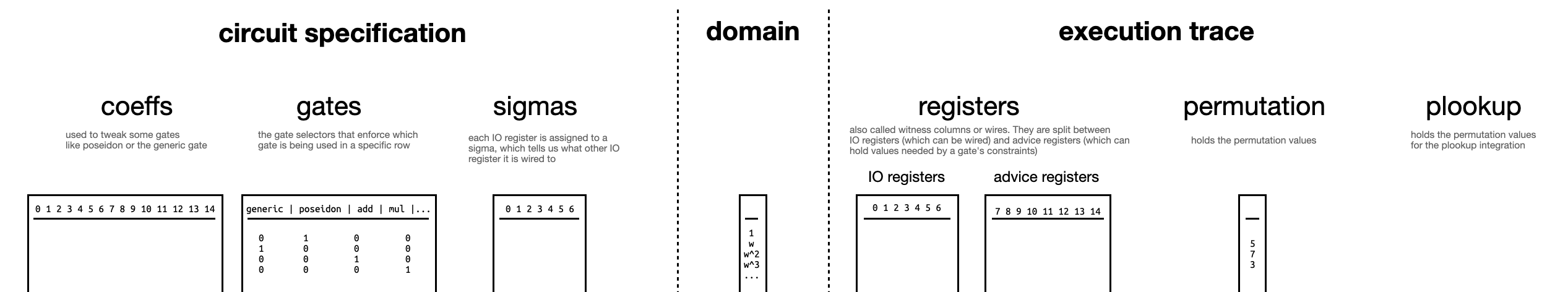
Glossary

Size: number of rows
Columns: number of variables per rows
Cell: a pair (row, column)
Witness: the values assigned in all the cells
Gate: polynomials that act on the variables in a row
Selector vector: a vector of values 1 or 0 (not true for constant vector I think) that toggles gates and variables in a row
Gadget: a series of contiguous rows with some specific gates set (via selector vectors)

Domain

$P l o n K$ needs a domain to encode the circuit on (for each point we can encode a row/constraint/gate). We choose a domain $H$ such that it is a multiplicative subgroup of the scalar field of our curve.

2-adicity

Furthermore, as FFT (used for interpolation, see the section on FFTs) works best in domains of size $2^{k}$ for some $k$ , we choose $H$ to be a subgroup of order $2^{k}$ .

Since the pasta curves both have scalar fields of prime orders $p$ and $q$ , their multiplicative subgroup is of order $p - 1$ and $q - 1$ respectively (without the zero element). The pasta curves were generated specifically so that both $p - 1$ and $q - 1$ are multiples of $2^{32}$ .

We say that they have 2-adicity of 32.

Looking at the definition of one of the pasta fields in Rust you can see that it is defined specifically for a trait related to FFTs:

#![allow(unused)]
fn main() {
impl FftParameters for FqParameters {
    type BigInt = BigInteger;

    const TWO_ADICITY: u32 = 32;

    #[rustfmt::skip]
    const TWO_ADIC_ROOT_OF_UNITY: BigInteger = BigInteger([
        0x218077428c9942de, 0xcc49578921b60494, 0xac2e5d27b2efbee2, 0xb79fa897f2db056
    ]);
}

The 2-adicity of 32 means that there’s a multiplicative subgroup of size $2^{32}$ that exists in the field. The code above also defines a generator $g$ for it, such that $g^{2^{32}} = 1$ and $g^{i} \neq = 1$ for $i \in [[1, 2^{32} - 1]]$ (so it’s a primitive $2^{32}$ -th root of unity).

[Lagrange’s theorem](https://en.wikipedia.org/wiki/Lagrange%27s_theorem_(group_theory)) tells us that if we have a group of order $n$ , then we’ll have subgroups with orders dividing $n$ . So in our case, we have subgroups with all the powers of 2, up to the 32-th power of 2.

To find any of these groups, it is pretty straight forward as well. Notice that:

let $h = g^{2}$ , then $h^{2^{31}} = g^{2^{32}} = 1$ and so $h$ generates a subgroup of order 31
let $t = g^{2^{2}}$ , then $t^{2^{30}} = g^{2^{32}} = 1$ and so $t$ generates a subgroup of order 30
and so on…

In arkworks you can see how this is implemented:

#![allow(unused)]
fn main() {
let size = n.next_power_of_two() as u64;
let log_size_of_group = ark_std::log2(usize::try_from(size).expect("too large"));
omega = Self::TWO_ADIC_ROOT_OF_UNITY;
for _ in log_size_of_group..Self::TWO_ADICITY {
    omega.square_in_place();
}
}

this allows you to easily find subgroups of different sizes of powers of 2, which is useful in zero-knowledge proof systems as FFT optimizations apply well on domains that are powers of 2. You can read more about that in the mina book.

Efficient computation of the vanishing polynomial

For each curve, we generate a domain $H$ as the set $H = 1, ω, ω^{2}, \dots, ω^{n - 1}$ . As we work in a multiplicative subgroup, the polynomial that vanishes in all of these points can be written and efficiently calculated as $Z_{H} (x) = x^{∣ H ∣} - 1$ .
This is because, by definition, $ω^{∣ H ∣} = 1$ . If $x \in H$ , then $x = ω^{i}$ for some $i$ , and we have:

$x^{∣ H ∣} = (ω^{i})^{∣ H ∣} = (ω^{∣ H ∣})^{i} = 1^{i} = 1$

This optimization is important, as without it calculating the vanishing polynomial would take a number of operations linear in $∣ H ∣$ (which is not doable in a verifier circuit, for recursion). With the optimization, it takes us a logarithmic number of operation (using exponentiation by squaring) to calculate the vanishing polynomial.

Lagrange basis in multiplicative subgroups

What’s a lagrange base?

$L_{i} (x) = 1$ if $x = g^{i}$ , $0$ otherwise.

What’s the formula?

Arkworks has the formula to construct a lagrange base:

Evaluate all Lagrange polynomials at $τ$ to get the lagrange coefficients. Define the following as

$H$ : The coset we are in, with generator $g$ and offset $h$

$m$ : The size of the coset $H$

$Z_{H}$ : The vanishing polynomial for $H$ . $Z_{H} (x) = \prod_{i \in [m]} (x - h \cdot g^{i}) = x^{m} - h^{m}$

$v_{i}$ : A sequence of values, where $v_{0} = \frac{1}{m * h ^{m - 1}}$ , and $v_{i + 1} = g \cdot v_{i}$

We then compute $L_{i, H} (τ)$ as $L_{i, H} (τ) = Z_{H} (τ) \cdot \frac{v _{i}}{τ - h g ^{i}}$

However, if $τ$ in $H$ , both the numerator and denominator equal 0 when i corresponds to the value tau equals, and the coefficient is 0 everywhere else. We handle this case separately, and we can easily detect by checking if the vanishing poly is 0.

following this, for $h = 1$ we have:

$L_{0} (x) = \frac{Z _{H} ( x )}{m ( x - 1 )}$
$L_{1} (x) = \frac{Z _{H} ( x ) g}{m ( x - g )}$
$L_{2} (x) = \frac{Z _{H} ( x ) g ^{2}}{m ( x - g ^{2} )}$
and so on

What’s the logic here?

https://en.wikipedia.org/wiki/Lagrange_polynomial#Barycentric_form

Non-Interactivity via Fiat-Shamir

So far we’ve talked about an interactive protocol between a prover and a verifier. The zero-knowledge proof was also in the honest verifier zero-knowedlge (HVZK) model, which is problematic.

In practice, we want to remove the interaction and have the prover produce a proof by themselves, that anyone can verify.

Public-coin protocols

public-coin protocols are protocols were the messages of the verifier are simply random messages. This is important as our technique to transform an interactive protocol to a non-interactive protocol works on public-coin protocols.

Fiat-Shamir trick

The whole idea is to replace the verifier by a random oracle, which in practice is a hash function. Note that by doing this, we remove potential leaks that can happen when the verifier acts dishonestly.

Initially the Fiat-Shamir transformation was only applied to sigma protocols, named after the greek letter $Σ$ due to its shape resembling the direction of messages (prover sends a commit to a verifier, verifier sends a challenge to a prover, prover sends the final proof to a verifier). A $Z$ would have made more sense but here we are.

Generalization of Fiat-Shamir

As our protocol has more than three moves, where every even move is a challenge from the verifier, we need to generalize Fiat-Shamir. This is simple: every verifier move can be replaced by a hash of the transcript (every message sent and received so far) to obtain a challenge.

In practice: a duplex construction as Merlin

While we use a hash function for that, a different construction called the duplex construction is particularly useful in such situations as they allow to continuously absorb the transcript and produce challenges, while automatically authenticating the fact that they produced a challenge.

Merlin is a standardization of such a construction using the Strobe protocol framework (a framework to make use of a duplex construction). Note that the more recent Xoodyak (part of NIST’s lightweight competition) could have been used for this as well. Note also that Mina uses none of these standards, instead it simply uses Poseidon (see section on poseidon).

$Plookup$

$Plookup$ allows us to check if witness values belong to a look up table. This is usually useful for reducing the number of constraints needed for bit-wise operations. So in the rest of this document we’ll use the XOR table as an example.

A	B	Y
0	0	0
0	1	1
1	0	1
1	1	0

First, let’s define some terms:

lookup table: a table of values that means something, like the XOR table above
joint lookup table: a table where cols have been joined together in a single col (with a challenge)
table entry: a cell in a joint lookup table
single lookup value: a value we’re trying to look up in a table
joint lookup values: several values that have been joined together (with a challenge)

A joint lookup table looks like this, for some challenge $α$ :

joint lookup table

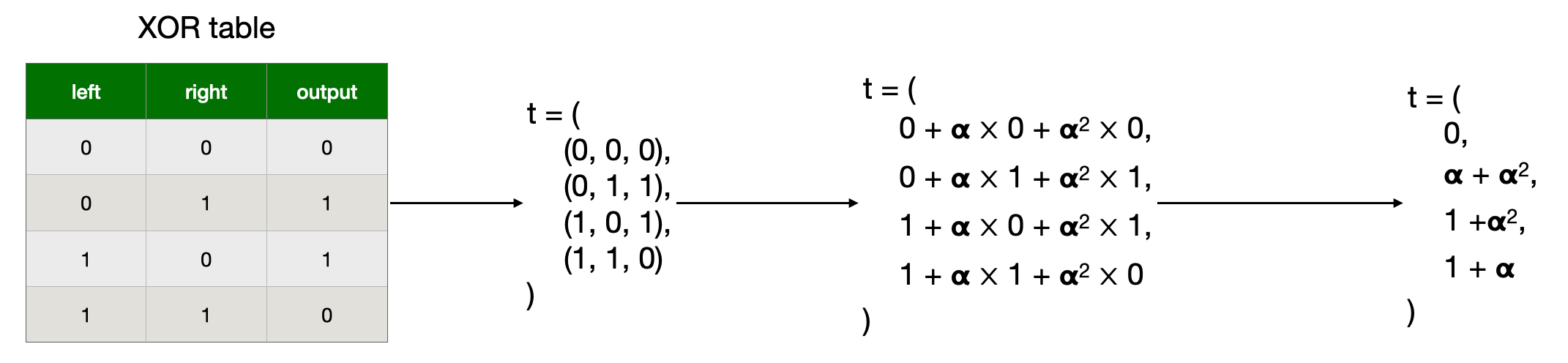
Constraints

Computes the aggregation polynomial for maximum $n$ lookups per row, whose $k$ -th entry is the product of terms:

$\frac{( γ ( 1 + β ) + t _{i} + β t _{i + 1} ) \prod _{j = 0}^{n} (( 1 + β ) ( γ + f _{i, j} ))}{\prod _{j = 0}^{n + 1} ( γ ( 1 + β ) + s _{i, j} + β s _{i + 1, j} )}$

for $i < k$ .

$t_{i}$ is the $i$ -th entry in the table
$f_{i, j}$ is the $j$ -th lookup in the $i$ -th row of the witness

For every instance of a value in $t_{i}$ and $f_{i, j}$ , there is an instance of the same value in $s_{i, j}$

$s_{i, j}$ is sorted in the same order as $t_{i}$ , increasing along the ‘snake-shape’

Whenever the same value is in $s_{i, j}$ and $s_{i + 1, j}$ , that term in the denominator product becomes

$(1 + β) (γ + s_{i, j})$

this will cancel with the corresponding looked-up value in the witness

$(1 + β) (γ + f_{i, j})$

Whenever the values $s_{i, j}$ and $s_{i + 1, j}$ differ, that term in the denominator product will cancel with some matching

$(γ (1 + β) + t_{i^{'}} + β t_{i^{'} + 1})$

because the sorting is the same in $s$ and $t$ .

There will be exactly the same number of these as the number of values in $t$ if $f$ only contains values from $t$ . After multiplying all of the values, all of the terms will have cancelled if $s$ is a sorting of $f$ and $t$ , and the final term will be $1$ because of the random choice of $β$ and $γ$ , there is negligible probability that the terms will cancel if $s$ is not a sorting of $f$ and $t$

But because of the snakify:

we are repeating an element between cols, we need to check that it’s the same in a constraint
we invert the direction, but that shouldn’t matter

FAQ

how do we do multiple lookups per row?
how do we dismiss rows where there are no lookup?

Maller’s Optimization to Reduce Proof Size

In the $P l o n K$ paper, they make use of an optimization from Mary Maller in order to reduce the proof size.

Explanation

Maller’s optimization is used in the “polynomial dance” between the prover and the verifier to reduce the number of openings the prover send.

Recall that the polynomial dance is the process where the verifier and the prover form polynomials together so that:

the prover doesn’t leak anything important to the verifier
the verifier doesn’t give the prover too much freedom

In the dance, the prover can additionally perform some steps that will keep the same properties but with reduced communication.

Let’s see the protocol where Prover wants to prove to Verifier that

$\forall x \in F, h_{1} (x) h_{2} (x) - h_{3} (x) = 0$

given commitments of $h_{1}, h_{2}, h_{3}$ ,

maller 1

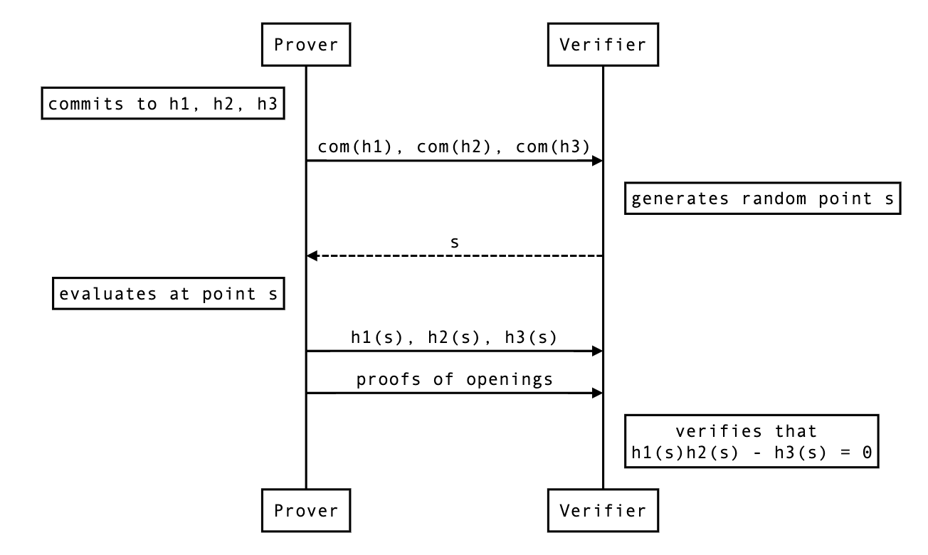
A shorter proof exists. Essentially, if the verifier already has the opening h1(s), they can reduce the problem to showing that

$\forall x \in F, L (x) = h_{1} (s) h_{2} (x) - h_{3} (x) = 0$

given commitments of $h_{1}, h_{2}, h_{3}$ and evaluation of $h 1$ at a point $s$ .

maller 2

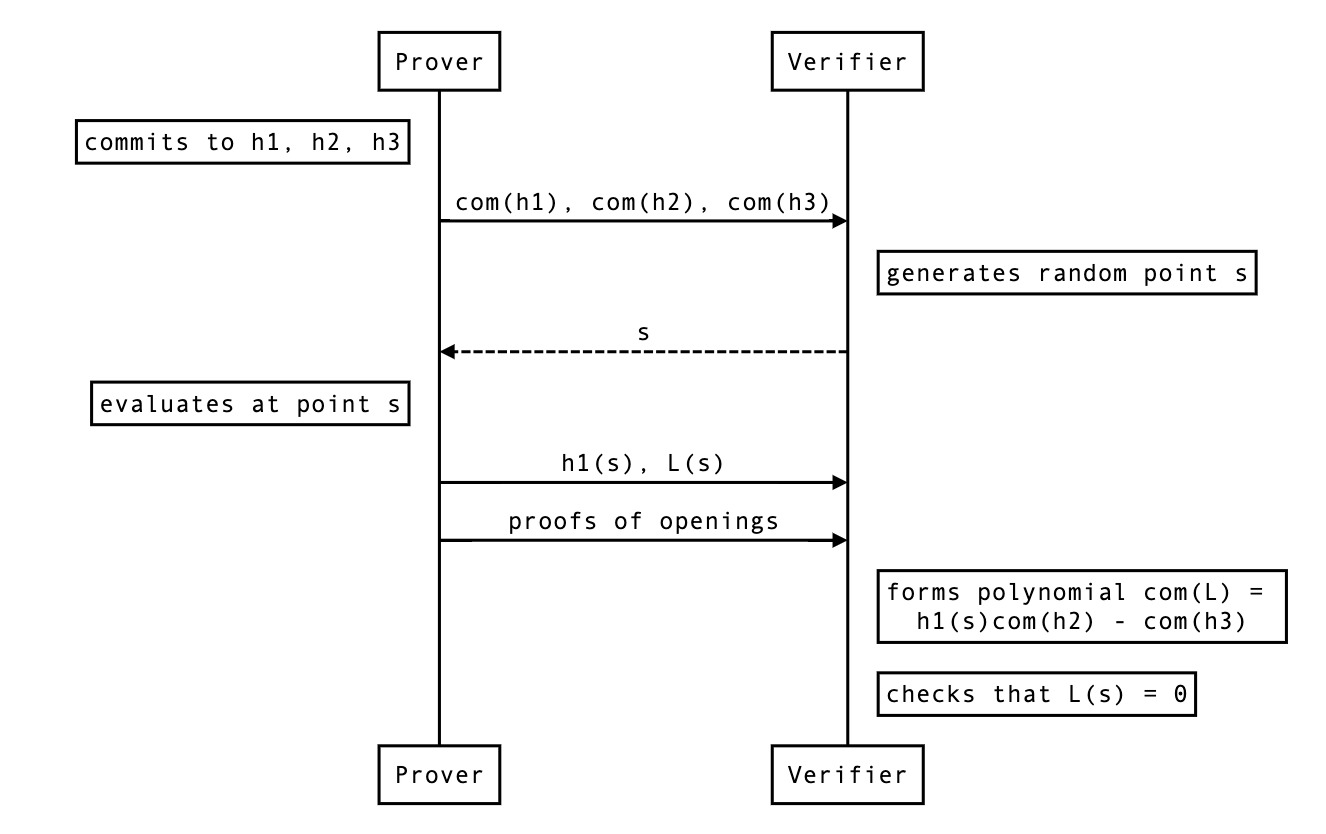
Notes

Why couldn’t the prover open the polynomial $L^{'}$ directly?

$L^{'} (x) = h_{1} (x) h_{2} (x) - h_{3} (x)$

By doing

maller 3

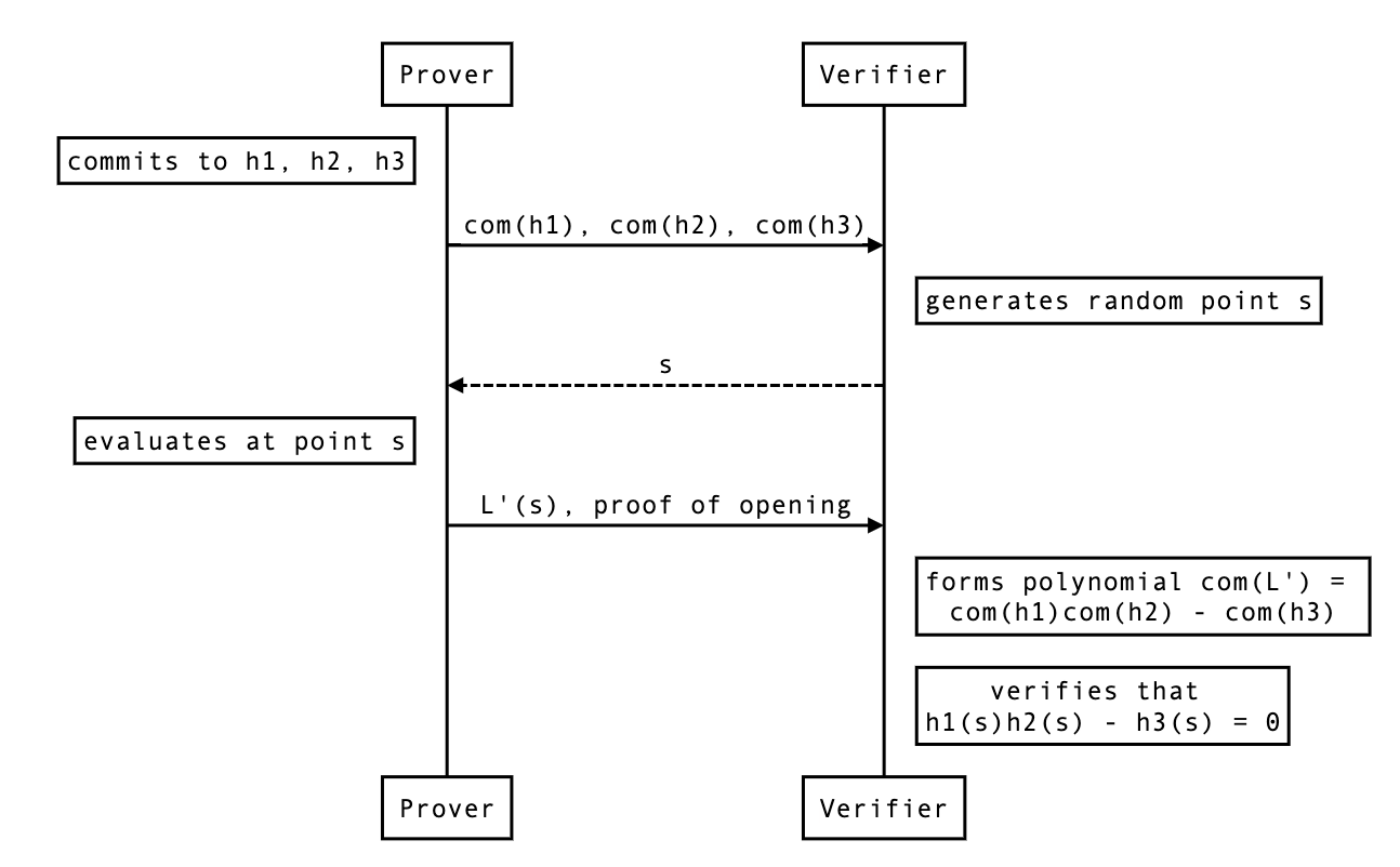
The problem here is that you can’t multiply the commitments together without using a pairing (if you’re using a pairing-based polynomial commitment scheme), and you can only use that pairing once in the protocol.

If you’re using an inner-product-based commitment, you can’t even multiply commitments.

question: where does the multiplication of commitment occurs in the pairing-based protocol of $P l o n K$ ? And how come we can use bootleproof if we need that multiplication of commitment?

Appendix: Original explanation from the $P l o n K$ paper

https://eprint.iacr.org/2019/953.pdf

For completion, the lemma 4.7:

A More Efficient Approach to Zero Knowledge for PLONK

In PLONK (considered as an interactive oracle proof), the prover sends the verifier several polynomials. They are evaluated at some $k$ points during the course of the protocol. Of course, if we want zero-knowledge, we would require that those evaluations do not reveal anything about the proof’s underlying witness.

PLONK as described here achieves zero knowledge by multiplying the polynomials with a small degree polynomial of random coefficients. When PLONK is instantiated with a discrete-log base Bootle et al type polynomial commitment scheme, the polynomial degrees must be padded to the nearest power of two. As a result, since several of the polynomials in PLONK already have degree equal to a power of two before the zero-knowledge masking, the multiplication with a random polynomial pushes the degree to the next power of two, which hurts efficiency. In order to avoid it, we propose an alternative method of achieving zero knowledge.

Zero Knowledge for the Column Polynomials

Let $w$ be the number of rows in a PLONK constraint system. For a typical real-world circuit, $w$ will not be equal to a power of two.

Let the witness elements from one column be $s_{1}, s_{2}, \dots, s_{w}$ . Let $n$ be the closest power of two to $w$ such that $n \geq w$ . Let $F$ be the field that witness elements belong to.

Now, in vanilla PLONK, we pad the $s_{i}$ with $n - w$ elements, interpolate the polynomial over a domain of size $n$ , scale it by a low degree random polynomial, and commit to the resulting polynomial. We want to avoid increasing the degree with the scaling by a low degree polynomial, so consider the following procedure.

Procedure. Sample $k$ elements uniformly from $F$ : $r_{w + 1}, \dots, r_{w + k}$ . Append them to the tuple of witness elements and then pad the remaining $n - (w + k)$ places as zeroes. The resulting tuple is interpolated as the witness polynomial. This approach ensures zero knowledge for the witness polynomials as established by Lemma 1.

Lemma 1. Let $H \subset F$ be a domain of size $n$ . Let $s_{1}, s_{2}, \dots, s_{w} \in F$ . Let $r_{w + 1}, \dots, r_{w + k}$ be $k$ uniformly and independently random elements in $F .$ Let $v$ be the $n$ -tuple $v = (s_{1}, s_{2}, \dots, s_{w}, r_{w + 1}, \dots, r_{w + k}, 0, \dots_{n - (w+k) times})$ . Let $f (X)$ be an interpolation polynomial of degree $n - 1$ such that $f (h_{i}) = v_{i}$ , where $h_{i} \in H$ . Let $c_{1}, \dots, c_{k}$ be any elements in $F$ such that $c_{i} \neq = v_{j}$ for every $i, j$ . Then, $(f (c_{1}), \dots, f (c_{k}))$ is distributed uniformly at random in $F^{k}$ .

Proof sketch. Recall that the interpolation polynomial is

$f (X) = j = 1 \sum n k \neq = j \prod \frac{( X - h _{k} )}{( h _{j} - h _{k} )} v_{j}$

With $V_{w + 1}, \dots, V_{w + k}$ as random variables, we have, $f (X) = a_{w + 1} V_{w + 1} + a_{w + 2} V_{w + 2} + \dots + a_{w + k} V_{w + k} + a$ for some constant field elements $a, a_{w + 1}, \dots, a_{w + k}$ . Therefore, assigning random values to $V_{w + 1}, \dots, V_{w + k}$ will give $k$ degrees of freedom that will let $(f (c_{1}), \dots, f (c_{k}))$ to be distributed uniformly at random in $F^{k}$ .

Zero Knowledge for the Permutation Polynomial

The other polynomial in PLONK for which we need zero-knowledge is the “permutation polynomial” $z$ . The idea here is to set the last $k$ evaluations to be uniformly random elements $t_{1}, \dots, t_{k}$ in $F$ . Then, we’ll modify the verification equation to not check for those values to satisfy the permutation property.

Modified permutation polynomial. Specifically, set $z (X)$ as follows.

$z (X) = L_{1} (X) + i = 1 \sum n - k - 2 (L_{i + 1} j = 1 \prod i frac_{i, j}) + t_{1} L_{n - k} (X) + \dots + t_{k} L_{n} (X)$

From Lemma 1, the above $z (X)$ has the desired zero knowledge property when $k$ evaluations are revealed. However, we need to modify the other parts of the protocol so that the last $k$ elements are not subject to the permutation evaluation, since they will no longer satisfy the permutation check. Specifically, we will need to modify the permutation polynomial to disregard those random elements, as follows.

$t (X) = (a (X) b (X) q_{M} (X) + a (X) q_{L} (X) + b (X) q_{R} (X) + c (X) q_{O} (X) + P I (X) + q_{C} (X)) \frac{1}{z _{H} ( X )} + ((a (X) + βX + γ) (b (X) + β k_{1} X + γ) (c (X) + β k_{2} X + γ) z (X) \times (X - h_{n - k}) \dots (X - h_{n - 1}) (X - h_{n})) \frac{α}{z _{H} ( X )} - ((a (X) + β S_{σ 1} (X) + γ) (b (X) + β S_{σ 2} (X) + γ) (c (X) + β S_{σ 3} (X) + γ) z (X ω) \times (X - h_{n - k}) \dots (X - h_{n - 1}) (X - h_{n})) \frac{α}{z _{H} ( X )} + (z (X) - 1) \cdot L_{1} (X) \frac{α ^{2}}{z _{H} ( X )} + (z (X) - 1) \cdot L_{n - k} (X) \frac{α ^{3}}{z _{H} ( X )}$

Modified permutation checks. To recall, the permutation check was originally as follows. For all $h \in H$ ,

$L_{1} (h) (Z (h) - 1) = 0$
$Z (h) [(a (h) + β h + γ) (b (h) + β k_{1} h + γ) (c (h) + β k_{2} h + γ)] = Z (ωh) [(a (h) + β S_{σ 1} (h) + γ) (b (h) + β S_{σ 2} (h) + γ) (c (h) + β S_{σ 3} (h) + γ)]$

The modified permuation checks that ensures that the check is performed only on all the values except the last $k$ elements in the witness polynomials are as follows.

For all $h \in H$ , $L_{1} (h) (Z (h) - 1) = 0$
For all $h \in H ∖ {h_{n - k}, \dots, h_{n}}$ , $Z (h) [(a (h) + β h + γ) (b (h) + β k_{1} h + γ) (c (h) + β k_{2} h + γ)] = Z (ωh) [(a (h) + β S_{σ 1} (h) + γ) (b (h) + β S_{σ 2} (h) + γ) (c (h) + β S_{σ 3} (h) + γ)]$
For all $h \in H$ , $L_{n - k} (h) (Z (h) - 1) = 0$

In the modified permutation polynomial above, the multiple $(X - h_{n - k}) \dots (X - h_{n - 1}) (X - h_{n})$ ensures that the permutation check is performed only on all the values except the last $k$ elements in the witness polynomials.

Overview

Here we explain how the Kimchi protocol design is translated into the proof-systems repository, from a high level perspective, touching briefly on all the involved aspects of cryptography. The concepts that we will be introducing can be studied more thoroughly by accessing the specific sections in the book.

In brief, the Kimchi protocol requires three different types of arguments Argument:

Custom gates: they correspond to each of the specific functions performed by the circuit, which are represented by gate constraints.
Permutation: the equality between different cells is constrained by copy constraints, which are represented by a permutation argument. It represents the wiring between gates, the connections from/to inputs and outputs.
Lookup tables: for efficiency reasons, some public information can be stored by both parties (prover and verifier) instead of wired in the circuit. Examples of these are boolean functions.

All of these arguments are translated into equations that must hold for a correct witness for the full relation. Equivalently, this is to say that a number of expressions need to evaluate to zero on a certain set of numbers. So there are two problems to tackle here:

Roots-check: Check that an equation evaluates to zero on a set of numbers.
Aggregation: Check that it holds for each of the equations.

Roots-check

For the first problem, given a polynomial $p (X)$ of degree $d$ , we are asking to check that $p (x) = 0$ for all $x \in S$ , where $S$ stands for set. Of course, one could manually evaluate each of the elements in the set and make sure of the above claim. But that would take so long (i.e. it wouldn’t be succinct). Instead, we want to check that all at once. And a great way to do it is by using a vanishing polynomial. Such a polynomial $v_{S} (X)$ will be nothing else than the smallest polynomial that vanishes on $S$ . That means, it is exactly defined as the degree $∣ S ∣$ polynomial formed by the product of the monomials:

$v_{S} (X) = s \in S \prod (X - s)$

And why is this so advantageous? Well, first we need to make a key observation. Since the vanishing polynomial equals zero on every $x \in S$ , and it is the smallest such polynomial (recall it has the smallest possible degree so that this property holds), if our initial polynomial $p (X)$ evaluates to zero on $S$ , then it must be the case that $p (X)$ is a multiple of the vanishing polynomial $v_{S} (X)$ . But what does this mean in practice? By polynomial division, it simply means there exists a quotient polynomial of degree $d - ∣ S ∣$ such that:

$q (X) := \frac{p ( X )}{v _{S} ( X )}$

And still, where’s the hype? If you can provide such a quotient polynomial, one could easily check that if $q (a) = p (a) / v_{S} (a)$ for a random number $a \in F$ \ $S$ (recall you will check in a point out of the set, otherwise you would get a $0/0$ ), then with very high probability that would mean that actually $p (X) = q (X) \cdot v_{S} (X)$ , meaning that $p (X)$ vanishes on the whole set $S$ , with just one point!

Let’s take a deeper look into the “magic” going on here. First, what do we mean by high probability? Is this even good enough? And the answer to this question is: as good as you want it to be.

First we analyse the math in this check. If the polynomial form of $p (X) = q (X) \cdot v_{S} (X)$ actually holds, then of course for any possible $a \in F$ \ $S$ the check $p (a) =_{?} q (a) \cdot v_{S} (a)$ will hold. But is there any unlucky instantiation of the point $a$ such that $p (a) = q (a) \cdot v_{S} (a)$ but $p (X) \neq = q (X) \cdot v_{S} (X)$ ? And the answer is, yes, there are, BUT not many. But how many? How unlikely this is? You already know the answer to this: Schwartz-Zippel. Recalling this lemma:

Given two different polynomials $f (X)$ and $g (X)$ of degree $d$ , they can at most intersect (i.e. coincide) in $d$ points. Or what’s equivalent, let $h (X) := f (X) - g (X)$ , the polynomial $h (X)$ can only evaluate to $0$ in at most $d$ points (its roots).

Thus, if we interchange $p (X) \to f (X)$ and $q (X) \cdot v_{S} (X) \to g (X)$ , both of degree $d$ , there are at most $\frac{d}{∣ F - S ∣}$ unlucky points of $a$ that could trick you into thinking that $p (X)$ was a multiple of the vanishing polynomial (and thus being equal to zero on all of $S$ ). So, how can you make this error probability negligible? By having a field size that is big enough (the formal definition says that the inverse of its size should decrease faster than any polynomial expression). Since we are working with fields of size $2^{255}$ , we are safe on this side!

Second, is this really faster than checking that $p (x) = 0$ for all $x \in S$ ? At the end of the day, it seems like we need to evaluate $v_{S} (a)$ , and since this is a degree $∣ S ∣$ polynomial it looks like we are still performing about the same order of computations. But here comes math again. In practice, we want to define this set $S$ to have a nice structure that allows us to perform some computations more efficiently than with arbitrary sets of numbers. Indeed, this set will normally be a multiplicative group (normally represented as $G$ or $H$ ), because in such groups the vanishing polynomial $v_{G} (X) := \prod_{ω \in G} (X - ω)$ has an efficient representation $v_{G} (X) = X^{∣ G ∣} - 1$ , which is much faster to evaluate than the above product.

Third, we may want to understand what happens with the evaluation of $p (a)$ instead. Since this is a degree $d \geq ∣ G ∣$ , it may look like this will as well take a lot of effort. But here’s where cryptography comes into play, since the verifier will never get to evaluate the actual polynomial by themselves. Various reasons why. One, if the verifier had access to the full polynomial $p (X)$ , then the prover should have sent it along with the proof, which would require $d + 1$ coefficients to be represented (and this is no longer succinct for a SNARK). Two, this polynomial could carry some secret information, and if the verifier could recompute evaluations of it, they could learn some private data by evaluating on specific points. So instead, these evaluations will be a “mental game” thanks to polynomial commitments and proofs of evaluation sent by the prover (for whom a computation in the order of $d$ is not only acceptable, but necessary). The actual proof length will depend heavily on the type of polynomial commitments we are using. For example, in Kate-like commitments, committing to a polynomial takes a constant number of group elements (normally one), whereas in Bootleproof it is logarithmic. But in any case this will be shorter than sending $O (d)$ elements.

Aggregation

So far we have seen how to check that a polynomial equals zero on all of $G$ , with just a single point. This is somehow an aggregation per se. But we are left to analyse how we can prove such a thing, for many polynomials. Altogether, if they hold, this will mean that the polynomials encode a correct witness and the relation would be satisfied. These checks can be performed one by one (checking that each of the quotients are indeed correct), or using an efficient aggregation mechanism and checking only one longer equation at once.

So what is the simplest way one could think of to perform this one-time check? Perhaps one could come up with the idea of adding up all of the equations $p_{0} (X), \dots, p_{n} (X)$ into a longer one $\sum_{i = 0}^{n} p_{i} (X)$ . But by doing this, we may be cancelling out terms and we could get an incorrect statemement.

So instead, we can multiply each term in the sum by a random number. The reason why this trick works is the independence between random numbers. That is, if two different polynomials $f (X)$ and $g (X)$ are both equal to zero on a given $X = x$ , then with very high probability the same $x$ will be a root of the random combination $α \cdot f (x) + β \cdot g (x) = 0$ . If applied to the whole statement, we could transform the $n$ equations into a single equation,

$i_{n} ⋀ p_{i} (X) =_{?} 0 \Leftrightarrow_{w . h . p .} i = 0 \sum n ρ_{i} \cdot p_{i} (X) =_{?} 0$

This sounds great so far. But we are forgetting about an important part of proof systems which is proof length. For the above claim to be sound, the random values used for aggregation should be verifier-chosen, or at least prover-independent. So if the verifier had to communicate with the prover to inform about the random values being used, we would get an overhead of $n$ field elements.

Instead, we take advantage of another technique that is called powers-of-alpha. Here, we make the assumption that powers of a random value $α^{i}$ are indistinguishable from actual random values $ρ_{i}$ . Then, we can twist the above claim to use only one random element $α$ to be agreed with the prover as:

$i_{n} ⋀ p_{i} (X) =_{?} 0 \Leftrightarrow_{w . h . p .} i = 0 \sum n α^{i} \cdot p_{i} (X) =_{?} 0$

Arguments

In the previous section we saw how we can prove that certain equations hold for a given set of numbers very efficiently. What’s left to understand is the motivation behind these techniques. Why is it so important that we can perform these operations and what do these equations represent in the real world?

But first, let’s recall the table that summarizes some important notation that will be used extensively: kimchi

One of the first ideas that we must grasp is the notion of a circuit. A circuit can be thought of as a set of gates with wires connections between them. The simplest type of circuit that one could think of is a boolean circuit. Boolean circuits only have binary values: $1$ and $0$ , true and false. From a very high level, boolean circuits are like an intricate network of pipes, and the values could be seen as water or no water. Then, gates will be like stopcocks, making water flow or not between the pipes. This video is a cool representation of this idea. Then, each of these behaviours will represent a gate (i.e. logic gates). One can have circuits that can perform more operations, for instance arithmetic circuits. Here, the type of gates available will be arithmetic operations (additions and multiplications) and wires could have numeric values and we could perform any arbitrary computation.

But if we loop the loop a bit more, we could come up with a single Generic gate that could represent any arithmetic operation at once. This thoughtful type of gate is the one gate whose concatenation is used in Plonk to describe any relation. Apart from it’s wires, these gates are tied to an array of coefficients that help describe the functionality. But the problem of this gate is that it takes a large set of them to represent any meaningful function. So instead, recent Plonk-like proof systems have appeared which use custom gates to represent repeatedly used functionalities more efficiently than as a series of generic gates connected to each other. Kimchi is one of these protocols. Currently, we give support to specific gates for the Poseidon hash function, the CompleteAdd operation for curve points, VarBaseMul for variable base multiplication, EndoMulScalar for endomorphism variable base scalar multiplication, RangeCheck for range checks and ForeignFieldMul and ForeignFieldAdd for foreign field arithmetic. Nonetheless, we have plans to further support many other gates soon, possibly even Cairo instructions.

The circuit structure is known ahead of time, as this is part of the public information that is shared with the verifier. What is secret is what we call the witness of the relation, which is the correct instantiation of the wires of the circuit satisfying all of the checks. This means the verifier knows what type of gate appears in each part of the circuit, and the coefficients that are attached to each of them.

The execution trace refers to the state of all the wires throughout the circuit, upon instantiation of the witness. It will be represented as a table where the rows correspond to each gate and the columns refer to the actual wires of the gate (a.k.a. input and output registers) and some auxiliary values needed for the computation (a.k.a. advice registers). The current implementation of Kimchi considers a total of 15 columns with the first 7 columns corresponding to I/O registers. Additionally, gates are allowed to access the elements in the current row Curr and the next Next. The permutation argument acts on the I/O registers (meaning, it will check that the cells in the first 7 columns of the execution trace will be copied correctly to their destination cells). For this reason, these checks are also known as copy constraints.

Going back to the main motivation of the scheme, recall that we wanted to check that certain equations hold in a given set of numbers. Here’s where this claim starts to make sense. The total number of rows in the execution trace will give us a domain. That is, we define a mapping between each of the row indices of the execution trace and the elements of a multiplicative group $G$ with as many elements as rows in the table. Two things to note here. First, if no such group exists we can pad with zeroes. Second, any multiplicative group has a generator $g$ whose powers generate the whole group. Then we can assign to each row a power of $g$ . Why do we want to do this? Because this will be the set over which we want to check our equations: we can transform a claim about the elements of a group to a claim like “these properties hold for each of the rows of this table”. Interesting, right?

Understanding the implementation of the $f (ζ) = Z_{H} (ζ) t (ζ)$ check

Unlike the latest version of vanilla $P l o n K$ that implements the final check using a polynomial opening (via Maller’s optimization), we implement it manually. (That is to say, Izaak implemented Maller’s optimization for 5-wires.)

But the check is not exactly $f (ζ) = Z_{H} (ζ) t (ζ)$ . This note describes how and why the implementation deviates a little.

What’s f and what’s missing in the final equation?

If you look at how the evaluation of $f (z)$ is computed on the prover side (or the commitment of $f$ is computed on the verifier side), you can see that f is missing two things:

the public input part
some terms in the permutation

What is it missing in the permutation part? Let’s look more closely. This is what we have:

$- 1 \cdot \cdot \cdot \cdot \cdot \cdot \cdot \cdot z (ζ ω) \cdot zkpm (ζ) \cdot α^{PERM0} (w [0] (ζ) + β \cdot σ [0] (ζ) + γ) (w [1] (ζ) + β \cdot σ [1] (ζ) + γ) (w [2] (ζ) + β \cdot σ [2] (ζ) + γ) (w [3] (ζ) + β \cdot σ [3] (ζ) + γ) (w [4] (ζ) + β \cdot σ [4] (ζ) + γ) (w [5] (ζ) + β \cdot σ [5] (ζ) + γ) β \cdot σ [6] (x)$

In comparison, here is the list of the stuff we needed to have:

the two sides of the coin: $z (ζ) \cdot \cdot \cdot \cdot \cdot \cdot \cdot \cdot zkpm (ζ) \cdot α^{PERM0} (w [0] (ζ) + β \cdot shift [0] (ζ) + γ) (w [1] (ζ) + β \cdot shift [1] (ζ) + γ) (w [2] (ζ) + β \cdot shift [2] (ζ) + γ) (w [3] (ζ) + β \cdot shift [3] (ζ) + γ) (w [4] (ζ) + β \cdot shift [4] (ζ) + γ) (w [5] (ζ) + β \cdot shift [5] (ζ) + γ) (w [6] (ζ) + β \cdot shift [6] (ζ) + γ)$ with $shift [0] = 1$
and $- 1 \cdot \cdot \cdot \cdot \cdot \cdot \cdot \cdot z (ζ ω) \cdot zkpm (ζ) \cdot α^{PERM0} (w [0] (ζ) + β \cdot σ [0] (ζ) + γ) (w [1] (ζ) + β \cdot σ [1] (ζ) + γ) (w [2] (ζ) + β \cdot σ [2] (ζ) + γ) (w [3] (ζ) + β \cdot σ [3] (ζ) + γ) (w [4] (ζ) + β \cdot σ [4] (ζ) + γ) (w [5] (ζ) + β \cdot σ [5] (ζ) + γ) (w [6] (ζ) + β \cdot σ [6] (ζ) + γ)$
the initialization: $(z (ζ) - 1) \cdot L_{1} (ζ) \cdot α^{PERM1}$
and the end of the accumulator: $(z (ζ) - 1) \cdot L_{n - k} (ζ) \cdot α^{PERM2}$

You can read more about why it looks like that in this post.

We can see clearly that the permutation stuff we have in f is clearly lacking. It’s just the subtraction part (equation 2), and even that is missing some terms. It is missing exactly this:

So at the end, when we have to check for the identity $f (ζ) = Z_{H} (ζ) t (ζ)$ we’ll actually have to check something like this (I colored the missing parts on the left hand side of the equation):

$f (ζ) + pub (ζ) + z (ζ) \cdot zkpm (ζ) \cdot α^{PERM0} \cdot (w [0] (ζ) + βζ + γ) \cdot (w [1] (ζ) + β \cdot shift [0] (ζ) + γ) \cdot (w [2] (ζ) + β \cdot shift [1] (ζ) + γ) \cdot (w [3] (ζ) + β \cdot shift [2] (ζ) + γ) \cdot (w [4] (ζ) + β \cdot shift [3] (ζ) + γ) \cdot (w [5] (ζ) + β \cdot shift [4] (ζ) + γ) \cdot (w [6] (ζ) + β \cdot shift [5] (ζ) + γ) - z (ζ ω) \cdot zkpm (ζ) \cdot α^{PERM0} \cdot \cdot (w [0] (ζ) + β \cdot σ [0] (ζ) + γ) \cdot \cdot (w [1] (ζ) + β \cdot σ [1] (ζ) + γ) \cdot \cdot (w [2] (ζ) + β \cdot σ [2] (ζ) + γ) \cdot \cdot (w [3] (ζ) + β \cdot σ [3] (ζ) + γ) \cdot \cdot (w [4] (ζ) + β \cdot σ [4] (ζ) + γ) \cdot \cdot (w [5] (ζ) + β \cdot σ [5] (ζ) + γ) \cdot \cdot (w [6] (ζ) + γ) + (z (ζ) - 1) \cdot L_{1} (ζ) \cdot α^{PERM1} + (z (ζ) - 1) \cdot L_{n - k} (ζ) \cdot α^{PERM2} = t (ζ) (ζ^{n} - 1)$

This is not exactly what happens in the code. But if we move things around a bit, we end up with what’s implemented. I highlight what changes in each steps. First, we just move things around:

$f (ζ) + pub (ζ) + z (ζ) \cdot zkpm (ζ) \cdot α^{PERM0} \cdot (w [0] (ζ) + β \cdot shift [0] ζ + γ) \cdot (w [1] (ζ) + β \cdot shift [1] ζ + γ) \cdot (w [2] (ζ) + β \cdot shift [2] ζ + γ) \cdot (w [3] (ζ) + β \cdot shift [3] ζ + γ) \cdot (w [4] (ζ) + β \cdot shift [4] ζ + γ) \cdot (w [5] (ζ) + β \cdot shift [5] ζ + γ) \cdot (w [6] (ζ) + β \cdot shift [6] ζ + γ) - z (ζ ω) \cdot zkpm (ζ) \cdot α^{PERM0} \cdot \cdot (w [0] (ζ) + β \cdot σ [0] (ζ) + γ) \cdot (w [1] (ζ) + β \cdot σ [1] (ζ) + γ) \cdot (w [2] (ζ) + β \cdot σ [2] (ζ) + γ) \cdot (w [3] (ζ) + β \cdot σ [3] (ζ) + γ) \cdot (w [4] (ζ) + β \cdot σ [4] (ζ) + γ) \cdot (w [5] (ζ) + β \cdot σ [5] (ζ) + γ) \cdot (w [6] (ζ) + γ) - t (ζ) (ζ^{n} - 1) = (1 - z (ζ)) L_{1} (ζ) α^{PERM1} + (1 - z (ζ)) L_{n - k} (ζ) α^{PERM2}$

here are the actual lagrange basis calculated with the formula here, oh and we actually use $L_{0}$ in the code, not $L_{1}$ , so let’s change that as well:

$f (ζ) + + - - = pub (ζ) z (ζ) \cdot zkpm (ζ) \cdot α^{PERM0} \cdot (w [0] (ζ) + β \cdot shift [0] ζ + γ) \cdot (w [1] (ζ) + β \cdot shift [1] ζ + γ) \cdot (w [2] (ζ) + β \cdot shift [2] ζ + γ) \cdot (w [3] (ζ) + β \cdot shift [3] ζ + γ) \cdot (w [4] (ζ) + β \cdot shift [4] ζ + γ) \cdot (w [5] (ζ) + β \cdot shift [5] ζ + γ) \cdot (w [6] (ζ) + β \cdot shift [6] ζ + γ) + z (ζ ω) \cdot zkpm (ζ) \cdot α^{PERM0} \cdot (w [0] (ζ) + β \cdot σ [0] (ζ) + γ) \cdot (w [1] (ζ) + β \cdot σ [1] (ζ) + γ) \cdot (w [2] (ζ) + β \cdot σ [2] (ζ) + γ) \cdot (w [3] (ζ) + β \cdot σ [3] (ζ) + γ) \cdot (w [4] (ζ) + β \cdot σ [4] (ζ) + γ) \cdot (w [5] (ζ) + β \cdot σ [5] (ζ) + γ) \cdot (w [6] (ζ) + γ) + t (ζ) (ζ^{n} - 1) (1 - z (ζ)) [\frac{( ζ ^{n} - 1 )}{n ( ζ - 1 )} α^{PERM1} + \frac{ω ^{n - k} ( ζ ^{n} - 1 )}{n ( ζ - ω ^{n - k} )} α^{PERM2}]$

finally we extract some terms from the lagrange basis:

$[f (ζ) + pub (ζ) + z (ζ) \cdot zkpm (ζ) \cdot α^{PERM0} \cdot (w [0] (ζ) + β \cdot shift [0] ζ + γ) \cdot (w [1] (ζ) + β \cdot shift [1] ζ + γ) \cdot (w [2] (ζ) + β \cdot shift [2] ζ + γ) \cdot (w [3] (ζ) + β \cdot shift [3] ζ + γ) \cdot (w [4] (ζ) + β \cdot shift [4] ζ + γ) \cdot (w [5] (ζ) + β \cdot shift [5] ζ + γ) \cdot (w [6] (ζ) + β \cdot shift [6] ζ + γ) + - z (ζ ω) \cdot zkpm (ζ) \cdot α^{PERM0} \cdot (w [0] (ζ) + β \cdot σ [0] (ζ) + γ) \cdot (w [1] (ζ) + β \cdot σ [1] (ζ) + γ) \cdot (w [2] (ζ) + β \cdot σ [2] (ζ) + γ) \cdot (w [3] (ζ) + β \cdot σ [3] (ζ) + γ) \cdot (w [4] (ζ) + β \cdot σ [4] (ζ) + γ) \cdot (w [5] (ζ) + β \cdot σ [5] (ζ) + γ) \cdot (w [6] (ζ) + γ) - t (ζ) (ζ^{n} - 1)] \cdot (ζ - 1) (ζ - ω^{n - k}) = (1 - z (ζ)) [\frac{( ζ ^{n} - 1 ) ( ζ - ω ^{n - k} )}{n} α^{PERM1} + \frac{ω ^{n - k} ( ζ ^{n} - 1 ) ( ζ - 1 )}{n} α^{PERM2}]$

with $α^{PERM0} = α^{17}, α^{PERM1} = α^{18}, α^{PERM2} = α^{19}$

Why do we do things this way? Most likely to reduce

Also, about the code:

the division by $n$ in the $α^{PERM1}$ and the $α^{PERM2}$ terms is missing (why?)
the multiplication by $w^{n - k}$ in the $α^{PERM2}$ term is missing (why?)

As these terms are constants, and do not prevent the division by $Z_{H}$ to form $t$ , $t$ also omits them. In other word, they cancel one another.

What about $t$ ?

In verifier.rs you can see the following code (cleaned to remove anything not important)

#![allow(unused)]
fn main() {
// compute the witness polynomials $w_0, \cdots, w_14$ and the permutation polynomial $z$ in evaluation forms on different domains
let lagrange = index.cs.evaluate(&w, &z);

// compute parts of the permutation stuff that is included in t
let (perm, bnd) = index.cs.perm_quot(&lagrange, &oracles, &z, &alpha[range::PERM])?;

// divide contributions with vanishing polynomial
let (mut t, res) = (perm + some_other_stuff).divide_by_vanishing_poly()

// add the other permutation stuff
t += &bnd;

// t is evaluated at zeta and sent...
}

Notice that bnd is not divided by the vanishing polynomial. Also what’s perm? Let’s answer the latter TESTREMOVEME:

$perm (x) = - a^{PERM0} \cdot zkpl (x) \cdot [z (x) \cdot (w [0] (x) + γ + x \cdot β \cdot shift [0]) \cdot (w [1] (x) + γ + x \cdot β \cdot shift [1]) \cdot \dots z (x \cdot w) \cdot (w [0] (x) + γ + σ [0] \cdot β) \cdot (w [1] (x) + γ + σ [1] \cdot β) \cdot \dots]$

and bnd is:

$bnd (x) = a^{PERM1} \cdot \frac{z ( x ) - 1}{x - 1} + a^{PERM2} \cdot \frac{z ( x ) - 1}{x - sid [ n - k ]}$

you can see that some terms are missing in bnd, specifically the numerator $x^{n} - 1$ . Well, it would have been cancelled by the division by the vanishing polynomial, and this is the reason why we didn’t divide that term by $Z_{H} (x) = x^{n} - 1$ .

Also, note that the same constant terms that were missing in $f$ are missing in $t$ .

Maller’s optimization for Kimchi

This document proposes a protocol change for kimchi.

What is Maller’s optimization?

See the section on Maller’s optimization for background.

Overview

We want the verifier to form commitment to the following polynomial:

$L (x) = f (x) - Z_{H} (ζ) \cdot t (x)$

They could do this like so:

$com (L) = com (f) - Z_{H} (ζ) \cdot com (t)$

Since they already know $f$ , they can produce $com (f)$ , the only thing they need is $com (t)$ . So the protocol looks like that:

maller 15 1

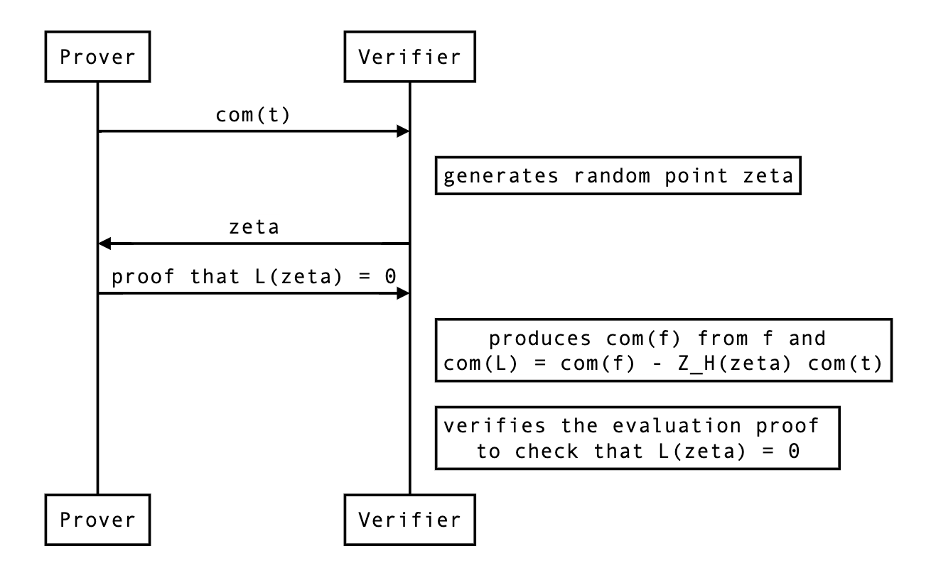
In the rest of this document, we review the details and considerations needed to implement this change in kimchi.

How to deal with a chunked $t$ ?

There’s one challenge that prevents us from directly using this approach: $com (t)$ is typically sent and received in several commitments (called chunks or segments throughout the codebase). As $t$ is the largest polynomial, usually exceeding the size of the SRS (which is by default set to be the size of the domain).

The verifier side

Thus, the verifier will have to produce split commitments of $L$ and combine them with powers of $ζ^{n}$ to verify an evaluation proof. Let’s define $L$ as:

$L = L_{0} + x^{n} L_{1} + x^{2 n} L_{1} + \dots$

where every $L_{i}$ is of degree $n - 1$ at most. Then we have that

$com (L) = com (L_{0}) + com (x^{n} \cdot L_{1}) + com (x^{2 n} \cdot L_{2}) + \dots$

Which the verifier can’t produce because of the powers of $x^{n}$ , but we can linearize it as we already know which $x$ we’re going to evaluate that polynomial with:

$com (\tilde{L}) = com (L_{0}) + ζ^{n} \cdot com (L_{1}) + ζ^{2 n} \cdot com (L_{2}) + \dots$

The prover side

This means that the prover will produce evaluation proofs on the following linearized polynomial:

$\tilde{L} (x) = 1 \cdot L_{0} (x) + ζ^{n} \cdot L_{1} (x) + ζ^{2 n} \cdot L_{2} (x) + \dots$

which is the same as $L (x)$ only if evaluated at $ζ$ . As the previous section pointed out, we will need $L (ζ ω)$ and $L (ζ ω) \neq = L (ζ ω)$ .

Evaluation proof and blinding factors

To create an evaluation proof, the prover also needs to produce the blinding factor $r_{L}$ associated with the chunked commitment of:

$L = f - (ζ^{n} - 1) \tilde{t}$

To compute it, there are two rules to follow:

when two commitment are added together, their associated blinding factors get added as well: $com (a) + com (b) ⟹ r_{a} + r_{b}$
when scaling a commitment, its blinding factor gets scalled too: $n \cdot com (a) ⟹ n \cdot r_{a}$

As such, if we know $r_{f}$ and $r_{t}$ , we can compute:

$r_{L} = r_{f} + (ζ^{n} - 1) \cdot r_{\tilde{t}}$

The prover knows the blinding factor of the commitment to $t$ , as they committed to it. But what about $f$ ? They never commit to it really, and the verifier recreates it from scratch using:

The commitments we sent them. In the linearization process, the verifier actually gets rid of most prover commitments, except for the commitment to the last sigma commitment $S_{σ 6}$ . (TODO: link to the relevant part in the spec) As this commitment is public, it is not blinded.
The public commitments. Think commitment to selector polynomials or the public input polynomial. These commitments are not blinded, and thus do not impact the calculation of the blinding factor.
The evaluations we sent them. Instead of using commitments to the wires when recreating $f$ , the verifier uses the (verified) evaluations of these in $ζ$ . If we scale our commitment $com (z)$ with any of these scalars, we will have to do the same with $r_{z}$ .

Thus, the blinding factor of $L$ is $(ζ^{n} - 1) \cdot r_{t}$ .

The evaluation of $\tilde{L}$

The prover actually does not send a commitment to the full $f$ polynomial. As described in the last check section. The verifier will have to compute the evaluation of $\tilde{L} (ζ)$ because it won’t be zero. It should be equal to the following:

$f (ζ) - t (ζ) (ζ^{n} - 1) = \frac{1 - z ( ζ )}{( ζ - 1 ) ( ζ - ω ^{n - k} )} [\frac{( ζ ^{n} - 1 ) ( ζ - ω ^{n - k} )}{n} α^{PERM1} + \frac{ω ^{n - k} ( ζ ^{n} - 1 ) ( ζ - 1 )}{n} α^{PERM2}] - pub (ζ) - z (ζ) \cdot zkpm (ζ) \cdot α^{PERM0} \cdot (w [0] (ζ) + β \cdot shift [0] ζ + γ) \cdot (w [1] (ζ) + β \cdot shift [1] ζ + γ) \cdot (w [2] (ζ) + β \cdot shift [2] ζ + γ) \cdot (w [3] (ζ) + β \cdot shift [3] ζ + γ) \cdot (w [4] (ζ) + β \cdot shift [4] ζ + γ) \cdot (w [5] (ζ) + β \cdot shift [5] ζ + γ) \cdot (w [6] (ζ) + β \cdot shift [6] ζ + γ) + z (ζ ω) \cdot zkpm (ζ) \cdot α^{PERM0} \cdot (w [0] (ζ) + β \cdot σ [0] (ζ) + γ) \cdot (w [1] (ζ) + β \cdot σ [1] (ζ) + γ) \cdot (w [2] (ζ) + β \cdot σ [2] (ζ) + γ) \cdot (w [3] (ζ) + β \cdot σ [3] (ζ) + γ) \cdot (w [4] (ζ) + β \cdot σ [4] (ζ) + γ) \cdot (w [5] (ζ) + β \cdot σ [5] (ζ) + γ) \cdot (w [6] (ζ) + γ) +$

Because we use the inner product polynomial commitment, we also need:

$L (ζ ω) = f (ζ ω) - Z_{H} (ζ) \cdot \tilde{t} (ζ ω)$ Notice the $Z_{H} (ζ)$ . That evaluation must be sent as part of the proof as well.

The actual protocol changes

Now here’s how we need to modify the current protocol:

The evaluations $f (ζ), f (ζ ω), t (ζ), t (ζ ω)$ (and their corresponding evaluation proofs) don’t have to be part of the protocol anymore.
The prover must still send the chunked commitments to $t$ .
The prover must create a linearized polynomial $L$ by creating a linearized polynomial $f$ and a linearized polynomial $t$ and computing: $L = f + (ζ^{n} - 1) \cdot t$
While the verifier can compute the evaluation of $L (ζ)$ by themselves, they don’t know the evaluation of $L (ζ ω)$ , so the prover needs to send that.
The verifier must recreate $com (L)$ , the commitment to $L$ , themselves so that they can verify the evaluation proofs of both $L (ζ)$ and $L (ζ ω)$ .
The evaluation of $\tilde{L} (ζ ω)$ must be absorbed in both sponges (Fq and Fr).

maller 15 2

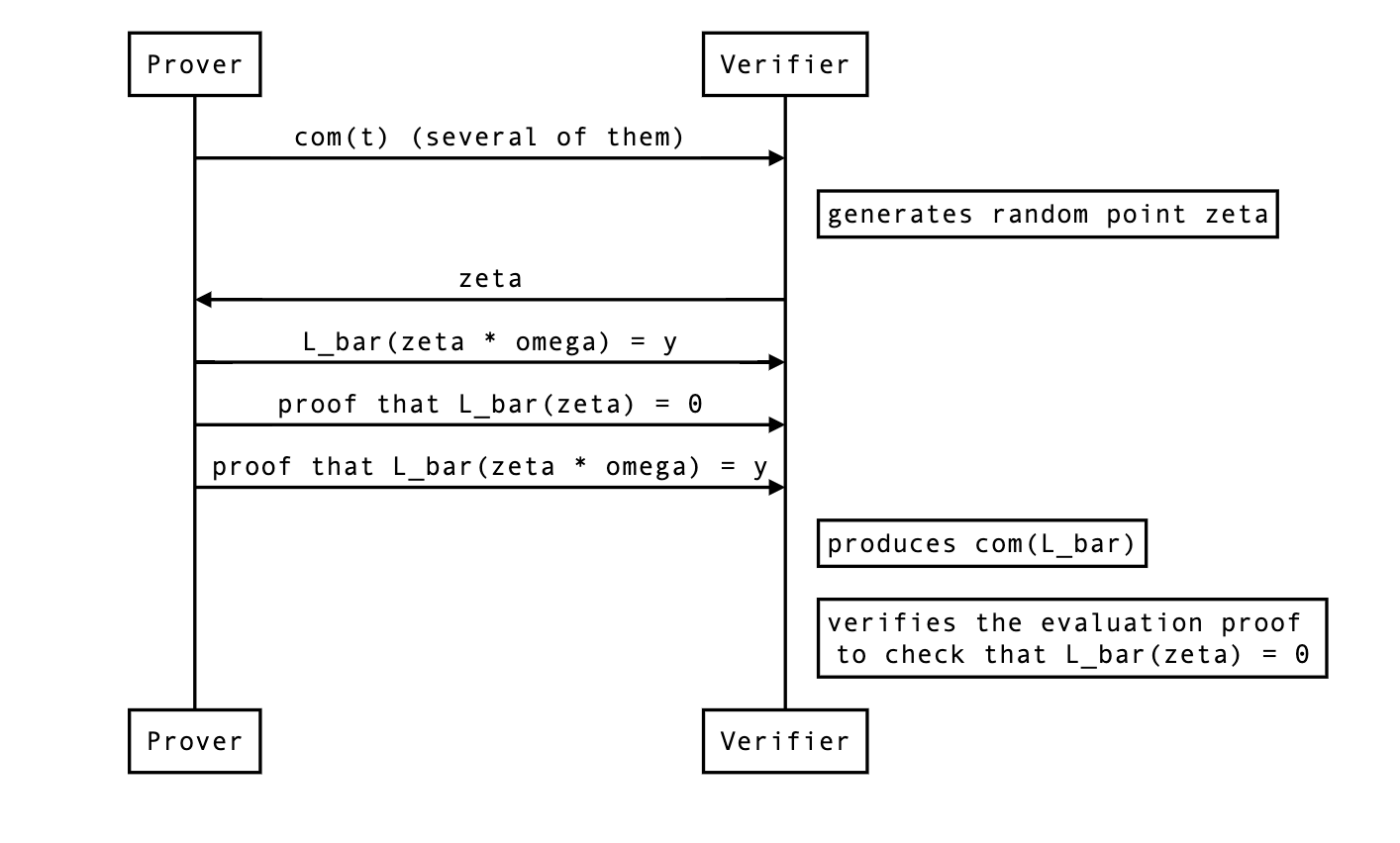
The proposal is implemented in #150 with the following details:

the $\tilde{L}$ polynomial is called ft.
the evaluation of $\tilde{L} (ζ)$ is called ft_eval0.
the evaluation $\tilde{L} (ζ ω)$ is called ft_eval1.

$Plookup$ in Kimchi

In 2020, $Plookup$ showed how to create lookup proofs. Proofs that some witness values are part of a lookup table. Two years later, an independent team published plonkup showing how to integrate $Plookup$ into $P l o n K$ .

This document specifies how we integrate $Plookup$ in kimchi. It assumes that the reader understands the basics behind $Plookup$ .

Overview

We integrate $Plookup$ in kimchi with the following differences:

we snake-ify the sorted table instead of wrapping it around (see later)
we allow fixed-ahead-of-time linear combinations of columns of the queries we make
we implemented different tables, like RangeCheck and XOR.
we allow several lookups (or queries) to be performed within the same row
zero-knowledgeness is added in a specific way (see later)

The following document explains the protocol in more detail

Recap on the grand product argument of $Plookup$

As per the $Plookup$ paper, the prover will have to compute three vectors:

$f$ , the (secret) query vector, containing the witness values that the prover wants to prove are part of the lookup table.
$t$ , the (public) lookup table.
$s$ , the (secret) concatenation of $f$ and $t$ , sorted by $t$ (where elements are listed in the order they are listed in $t$ ).

Essentially, $Plookup$ proves that all the elements in $f$ are indeed in the lookup table $t$ if and only if the following multisets are equal:

${(1 + β) f, diff (t)}$
$diff (sorted (f, t))$

where $diff$ is a new set derived by applying a “randomized difference” between every successive pairs of a vector, and $(f, t)$ is the set union of $f$ et $t$ .

More precisely, for a set $S = {s_{0}, s_{1}, \dots, s_{n}}$ , $diff (S)$ is defined as the set ${s_{0} + β s_{1}, s_{1} + β s_{2}, \dots, s_{n - 1} + β s_{n}}$ .

For example, with:

$f = {5, 4, 1, 5}$
$t = {1, 4, 5}$

we have:

$sorted (f, t) = {1, 1, 4, 4, 5, 5, 5}$
${(1 + β) f, diff (t)} = {(1 + β) 5, (1 + β) 4, (1 + β) 1, (1 + β) 5, 1 + β 4, 4 + β 5}$
$diff (sorted (f, t)) = {1 + β 1, 1 + β 4, 4 + β 4, 4 + β 5, 5 + β 5, 5 + β 5}$

Note: This assumes that the lookup table is a single column. You will see in the next section how to address lookup tables with more than one column.

The equality between the multisets can be proved with the permutation argument of $P l o n K$ , which would look like enforcing constraints on the following accumulator:

init: $acc_{0} = 1$
final: $acc_{n} = 1$
for every $0 < i \leq n$ : $acc_{i} = acc_{i - 1} \cdot \frac{( γ + ( 1 + β ) f _{i - 1} ) \cdot ( γ + t _{i - 1} + β t _{i} )}{( γ + s _{i - 1} + β s _{i} ) ( γ + s _{n + i - 1} + β s _{n + i} )}$

Note that the $Plookup$ paper uses a slightly different equation to make the proof work. It is possible that the proof would work with the above equation, but for simplicity let’s just use the equation published in $Plookup$ :

$acc_{i} = acc_{i - 1} \cdot \frac{( 1 + β ) \cdot ( γ + f _{i - 1} ) \cdot ( γ ( 1 + β ) + t _{i - 1} + β t _{i} )}{( γ ( 1 + β ) + s _{i - 1} + β s _{i} ) ( γ ( 1 + β ) + s _{n + i - 1} + β s _{n + i} )}$

Note: in $Plookup$ $s$ is longer than $n$ ( $∣ s ∣ = ∣ f ∣ + ∣ t ∣$ ), and thus it needs to be split into multiple vectors to enforce the constraint at every $i \in [[0; n]]$ . This leads to the two terms in the denominator as shown above, so that the degree of $γ (1 + β)$ is equal in the nominator and denominator.

Lookup tables

Kimchi uses different lookup tables, including RangeCheck and XOR. The XOR table for values of 1 bit is the following:

l	r	o
1	0	1
0	1	1
1	1	0
0	0	0

Whereas kimchi uses the XOR table for values of $4$ bits, which has $2^{8}$ entries.

Note: the $(0, 0, 0)$ entry is at the very end on purpose (as it will be used as dummy entry for rows of the witness that don’t care about lookups).

Querying the table

The $Plookup$ paper handles a vector of lookups $f$ which we do not have. So the first step is to create such a table from the witness columns (or registers). To do this, we define the following objects:

a query tells us what registers, in what order, and scaled by how much, are part of a query
a query selector tells us which rows are using the query. It is pretty much the same as a gate selector.

Let’s go over the first item in this section.

For example, the following query tells us that we want to check if $r_{0} \oplus r_{2} = 2 \cdot r_{1}$

l	r	o
1, $r_{0}$	1, $r_{2}$	2, $r_{1}$

$r_{0}$ , $r_{1}$ and $r_{2}$ will be the result of the evaluation at $g^{i}$ of respectively the wire polynomials $w_{0}$ , $w_{1}$ and $w_{2}$ . To perform vector lookups (i.e. lookups over a list of values, not a single element), we use a standard technique which consists of coining a combiner value $j$ and sum the individual elements of the list using powers of this coin.

The grand product argument for the lookup constraint will look like this at this point:

$acc_{i} = acc_{i - 1} \cdot \frac{( 1 + β ) \cdot ( γ + j ^{0} \cdot 1 \cdot w _{0} ( g ^{i} ) + j \cdot 1 \cdot w _{2} ( g ^{i} ) + j ^{2} \cdot 2 \cdot w _{1} ( g ^{i} )) \cdot ( γ ( 1 + β ) + t _{i - 1} + β t _{i} )}{( γ ( 1 + β ) + s _{i - 1} + β s _{i} ) ( γ ( 1 + β ) + s _{n + i - 1} + β s _{n + i} )}$

Not all rows need to perform queries into a lookup table. We will use a query selector in the next section to make the constraints work with this in mind.

Query selector

The associated query selector tells us on which rows the query into the XOR lookup table occurs.

row	query selector
0	1
1	0

Both the (XOR) lookup table and the query are built-ins in kimchi. The query selector is derived from the circuit at setup time.

With the selectors, the grand product argument for the lookup constraint has the following form:

$acc_{i} = acc_{i - 1} \cdot \frac{( 1 + β ) \cdot query \cdot ( γ ( 1 + β ) + t _{i - 1} + β t _{i} )}{( γ ( 1 + β ) + s _{i - 1} + β s _{i} )}$

where $query$ is constructed so that a dummy query ( $0 \oplus 0 = 0$ ) is used on rows that don’t have a query.

$query := selector \cdot (γ + j^{0} \cdot 1 \cdot w_{0} (g^{i}) + j \cdot 1 \cdot w_{2} (g^{i}) + j^{2} \cdot 2 \cdot w_{1} (g^{i})) + (1 - selector) \cdot (γ + 0 + j \cdot 0 + j^{2} \cdot 0)$

Supporting multiple queries

Since we would like to allow multiple table lookups per row, we define multiple queries, where each query is associated with a lookup selector.

Previously, ChaCha20 was implemented in Kimchi but has been removed as it has become unneeded. You can still find the implementation here. The ChaCha gates all perform $4$ queries in a row. Thus, $4$ is trivially the largest number of queries that happen in a row.

Important: to make constraints work, this means that each row must make $4$ queries. Potentially some or all of them are dummy queries.

For example, the ChaCha0, ChaCha1, and ChaCha2 gates will jointly apply the following 4 XOR queries on the current and following rows:

l	r	o	-	l	r	o	-	l	r	o	-	l	r	o
1, $r_{3}$	1, $r_{7}$	1, $r_{11}$	-	1, $r_{4}$	1, $r_{8}$	1, $r_{12}$	-	1, $r_{5}$	1, $r_{9}$	1, $r_{13}$	-	1, $r_{6}$	1, $r_{10}$	1, $r_{14}$

which you can understand as checking for the current and following row that

$r_{3} \oplus r_{7} r_{4} \oplus r_{8} r_{5} \oplus r_{9} r_{6} \oplus r_{10} = r_{11} = r_{12} = r_{13} = r_{14}$

The ChaChaFinal also performs $4$ (somewhat similar) queries in the XOR lookup table. In total this is $8$ different queries that could be associated to $8$ selector polynomials.

Grouping queries by queries pattern

Associating each query with a selector polynomial is not necessarily efficient. To summarize:

the ChaCha0, ChaCha1, and ChaCha2 gates that in total make $4$ queries into the XOR table
the ChaChaFinal gate makes another $4$ different queries into the XOR table

Using the previous section’s method, we’d have to use $8$ different lookup selector polynomials for each of the different $8$ queries. Since there’s only $2$ use-cases, we can simply group them by queries patterns to reduce the number of lookup selector polynomials to $2$ .

The grand product argument for the lookup constraint looks like this now:

$acc_{i} = acc_{i - 1} \cdot \frac{( 1 + β ) ^{4} \cdot query \cdot ( γ ( 1 + β ) + t _{i - 1} + β t _{i} )}{( γ ( 1 + β ) + s _{i - 1} + β s _{i} ) \times \dots}$

where $query$ is constructed as:

$query = selector_{1} \cdot pattern_{1} + selector_{2} \cdot pattern_{2} + (1 - selector_{1} - selector_{2}) \cdot (γ + 0 + j \cdot 0 + j^{2} \cdot 0)^{4}$

where, for example the first pattern for the ChaCha0, ChaCha1, and ChaCha2 gates looks like this:

$pattern_{1} = (γ + w_{3} (g^{i}) + j \cdot w_{7} (g^{i}) + j^{2} \cdot w_{11} (g^{i})) \cdot (γ + w_{4} (g^{i}) + j \cdot w_{8} (g^{i}) + j^{2} \cdot w_{12} (g^{i})) \cdot (γ + w_{5} (g^{i}) + j \cdot w_{9} (g^{i}) + j^{2} \cdot w_{13} (g^{i})) \cdot (γ + w_{6} (g^{i}) + j \cdot w_{10} (g^{i}) + j^{2} \cdot w_{14} (g^{i})) \cdot$

Note that there’s now $4$ dummy queries, and they only appear when none of the lookup selectors are active. If a pattern uses less than $4$ queries, it has to be padded with dummy queries as well.

Finally, note that the denominator of the grand product argument is incomplete in the formula above. Since the nominator has degree $5$ in $γ (1 + β)$ , the denominator must match too. This is achieved by having a longer $s$ , and referring to it $5$ times. The denominator thus becomes $\prod_{k = 1}^{5} (γ (1 + β) + s_{kn + i - 1} + β s_{kn + i})$ .

Back to the grand product argument

There are two things that we haven’t touched on:

The vector $t$ representing the combined lookup table (after its columns have been combined with a joint combiner $j$ ). The non-combined loookup table is fixed at setup time and derived based on the lookup tables used in the circuit.
The vector $s$ representing the sorted multiset of both the queries and the lookup table. This is created by the prover and sent as commitment to the verifier.

The first vector $t$ is quite straightforward to think about:

if it is smaller than the domain (of size $n$ ), then we can repeat the last entry enough times to make the table of size $n$ .
if it is larger than the domain, then we can either increase the domain or split the vector in two (or more) vectors. This is most likely what we will have to do to support multiple lookup tables later.

What about the second vector $s$ ?

The sorted vector $s$

We said earlier that in original $P l o n K$ the size of $s$ is equal to $∣ s ∣ = ∣ f ∣ + ∣ t ∣$ , where $f$ encodes queries, and $t$ encodes the lookup table. With our multi-query approach, the second vector $s$ is of the size

$n \cdot ∣# queries ∣ + ∣ lookup_table ∣$

That is, it contains the $n$ elements of each query vectors (the actual values being looked up, after being combined with the joint combinator, that’s $4$ per row), as well as the elements of our lookup table (after being combined as well).

Because the vector $s$ is larger than the domain size $n$ , it is split into several vectors of size $n$ . Specifically, in the plonkup paper, the two halves of $s$ , which are then interpolated as $h_{1}$ and $h_{2}$ . The denominator in $P l o n K$ in the vector form is $(γ (1 + β) + s_{i - 1} + β s_{i}) (γ (1 + β) + s_{n + i - 1} + β s_{n + i})$ which, when interpolated into $h_{1}$ and $h_{2}$ , becomes $(γ (1 + β) + h_{1} (x) + β h_{1} (g \cdot x)) (γ (1 + β) + h_{2} (x) + β h_{2} (g \cdot x))$

Since one has to compute the difference of every contiguous pairs, the last element of the first half is the replicated as the first element of the second half ( $s_{n - 1} = s_{n}$ ). Hence, a separate constraint must be added to enforce that continuity on the interpolated polynomials $h_{1}$ and $h_{2}$ :

$L_{n - 1} (X) \cdot (h_{1} (X) - h_{2} (g \cdot X)) \equiv 0$

which is equivalent to checking that $h_{1} (g^{n - 1}) = h_{2} (1)$ .

The sorted vector $s$ in kimchi

Since this vector is known only by the prover, and is evaluated as part of the protocol, zero-knowledge must be added to the corresponding polynomial (in case of $Plookup$ approach, to $h_{1} (X), h_{2} (X)$ ). To do this in kimchi, we use the same technique as with the other prover polynomials: we randomize the last evaluations (or rows, on the domain) of the polynomial.

This means two things for the lookup grand product argument:

We cannot use the wrap around trick to make sure that the list is split in two correctly (enforced by $L_{n - 1} (h_{1} (x) - h_{2} (g \cdot x)) = 0$ which is equivalent to $h_{1} (g^{n - 1}) = h_{2} (1)$ in the $Plookup$ paper)
We have even less space to store an entire query vector. Which is actually super correct, as the witness also has some zero-knowledge rows at the end that should not be part of the queries anyway.

The first problem can be solved in two ways:

Zig-zag technique. By reorganizing $s$ to alternate its values between the columns. For example, $h_{1} = (s_{0}, s_{2}, s_{4}, \dots)$ and $h_{2} = (s_{1}, s_{3}, s_{5}, \dots)$ so that you can simply write the denominator of the grand product argument as $(γ (1 + β) + h_{1} (x) + β h_{2} (x)) (γ (1 + β) + h_{2} (x) + β h_{1} (x \cdot g))$ Whis approach is taken by the plonkup paper.
Snake technique. By reorganizing $s$ as a snake. This is what is currently implemented in kimchi.

The snake technique rearranges $s$ into the following shape:

                           __    _
          s_0 |  s_{2n-1} |  |  | |
          ... |       ... |  |  | |
      s_{n-1} |       s_n |  |  | |
               ‾‾‾‾‾‾‾‾‾‾‾    ‾‾   ‾
              h1         h2  h3 ...

Assuming that for now we have only one bend and two polynomials $h_{1} (X), h_{2} (X)$ , the denominator has the following form:

$(γ (1 + β) + h_{1} (x) + β h_{1} (x \cdot g)) (γ (1 + β) + h_{2} (x \cdot g) + β h_{2} (x))$

and the snake doing a U-turn is constrained via $s_{n - 1} = s_{n}$ , enforced by the following equation:

$L_{n - 1} \cdot (h_{1} (x) - h_{2} (x)) = 0$

In practice, $s$ will have more sections than just two. Assume that we have $k$ sections in total, then the denominator generalizes to

$i = 1 \prod k γ (1 + β) + h_{i} (x \cdot g^{δ_{0, i mod 2}}) + β h_{i} (x \cdot g^{δ_{1, i mod 2}})$

where $δ_{i, j}$ is Kronecker delta, equal to $1$ when $i$ is even (for the first term) or odd (for the second one), and equal to $0$ otherwise.

Similarly, the U-turn constraints now become

$L_{n - 1} (X) \cdot (h_{2} (X) - h_{1} (X)) L_{0} (X) \cdot (h_{3} (X) - h_{2} (X)) L_{n - 1} (X) \cdot (h_{4} (X) - h_{3} (X)) \dots \equiv 0 \equiv 0 \equiv 0$

In our concrete case with $4$ simultaneous lookups the vector $s$ has to be split into $k = 5$ sections — each denominator term in the accumulator accounts for $4$ queries ( $f$ ) and $1$ table consistency check ( $t$ ).

Unsorted $t$ in $s$

Note that at setup time, $t$ cannot be sorted lexicographically as it is not combined yet. Since $s$ must be sorted by $t$ (in other words sorting of $s$ must follow the elements of $t$ ), there are two solutions:

Both the prover and the verifier can sort the combined $t$ lexicographically, so that $s$ can be sorted lexicographically too using typical sorting algorithms
The prover can directly sort $s$ by $t$ , so that the verifier doesn’t have to do any pre-sorting and can just rely on the commitment of the columns of $t$ (which the prover can evaluate in the protocol).

We take the second approach. However, this must be done carefully since the combined $t$ entries can repeat. For some $i, l$ such that $i \neq = l$ , we might have

$t_{0} [i] + j \cdot t_{1} [i] + j^{2} \cdot t_{2} [i] = t_{0} [l] + j \cdot t_{1} [l] + j^{2} \cdot t_{2} [l]$

For example, if $f = {1, 2, 2, 3}$ and $t = {2, 1, 2, 3}$ , then $sorted (f, t) = {2, 2, 2, 1, 1, 2, 3, 3}$ would be a way of correctly sorting the combined vector $s$ . At the same time $sorted (f, t) = {2, 2, 2, 2, 1, 1, 3, 3}$ is incorrect since it does not have a second block of $2$ s, and thus such an $s$ is not sorted by $t$ .

Recap

So to recap, to create the sorted polynomials $h_{i}$ , the prover:

creates a large query vector which contains the concatenation of the $4$ per-row (combined with the joint combinator) queries (that might contain dummy queries) for all rows
creates the (combined with the joint combinator) table vector
sorts all of that into a big vector $s$
divides that vector $s$ into as many $h_{i}$ vectors as a necessary following the snake method
interpolate these $h_{i}$ vectors into $h_{i}$ polynomials
commit to them, and evaluate them as part of the protocol.

Extended lookup tables

This (old) RFC proposes an extension to our use of lookup tables using the PLOOKUP multiset inclusion argument, so that values within lookup tables can be chosen after the constraint system for a circuit has been fixed.

Motivation

This extension should provide us with

array-style lookups (arr[i], where arr and i are formed of values in the proof witness).
the ability to load ‘bytecode’ using a proof-independent commitment.
the ability to load tables of arbitrary data for use in the circuit, allowing e.g. the full data of a HTTPS transcript to be entered into a proof without using some in-circuit commitment.
the ability to expose tables of arbitrary in-circuit data, for re-use by other proofs.

These goals support 5 major use-cases:

allow the verifier circuit to support ‘custom’ or user-specified gates
- using array indexing, the use of constants and commitments/evaluations can be determined by the verifier index, instead of being fixed by the permutation argument as currently.
allow random-access lookups in arrays as a base-primitive for user programs
allow circuits to use low-cost branching and other familiar programming primitives
- this depends on the development of a bytecode interpreter on top of the lookup-table primitives, where the values in the table represent the bytecode of the instructions.
allow circuits to load and execute some ‘user provided’ bytecode
- e.g. to run a small bytecode program provided in a transaction at block-production time.
allow zkOracles to load a full HTTPS transcript without using an expensive in-circuit commitment.

Detailed design

In order to support the desired goals, we first define 3 types of table:

fixed tables are tables declared as part of the constraint system, and are the same for every proof of that circuit.
runtime tables are tables whose contents are determined at proving time, to be used for array accesses to data from the witness. Also called dynamic tables in other projects.
side-loaded tables are tables that are committed to in a proof-independent way, so that they may be reused across proofs and/or signed without knowledge of the specific proof, but may be different for each execution of the circuit.

These distinct types of tables are a slight fiction: often it will be desirable to have some fixed part of runtime or side-loaded tables, e.g. to ensure that indexing is reliable. For example, a table representing an array of values [x, y, z] in the proof might be laid out as

value1	value2
0	?runtime
1	?runtime
2	?runtime

where the value1 entries are fixed in the constraint system. This ensure that a malicious prover is not free to create multiple values with the same index, such as [(0,a), (0,x), (1,y), (2,z)], otherwise the value a might be used where the value x was intended.

Combining multiple tables

The current implementation only supports a single fixed table. In order to make multiple tables available, we either need to run a separate PLOOKUP argument for each table, or to concatenate the tables to form an combined table and identify the values from each table in such a way that the prover cannot use values from the ‘wrong’ table.

We already solve a similar problem with ‘vector’ tables – tables where a row contains multiple values – where we want to ensure that the prover used an entry (x, y, z) from the table, and not some parts of different entries, or some other value entirely. In order to do this, we generate a randomising field element joint_combiner, where the randomness depends on the circuit witness, and then compute x + y * joint_combiner + z * joint_combiner^2. Notice that, if the prover wants to select some (a, b, c) not in the table and claim that it in fact was, they are not able to use the knowledge of the joint_combiner to choose their (a, b, c), since the joint_combiner will depend on those values a, b, and c.

This is a standard technique for checking multiple equalities at once by checking a single equality; to use it, we must simply ensure that the randomness depends on all of the (non-constant) values in the equality.

We propose extending each table with an extra column, which we will call the TableID column, which associates a different number with each table. Since the sizes of all tables must be known at constraint system time, we can treat this as a fixed column. For example, this converts a lookup (a, b, c) in the table with ID 1 into a lookup of (a, b, c, 1) in the combined table, and ensures that any value (x, y, z) from table ID 2 will not match that lookup, since its representative is (x, y, z, 2).

To avoid any interaction between the TableID column and any other data in the tables, we use TableID * joint_combiner^max_joint_size to mix in the TableID, where max_joint_size is the maximum length of any lookup or table value. This also simplifies the ‘joining’ of the table_id polynomial commitment, since we can straightforwardly scale it by the constant joint_combiner^max_joint_size to find its contribution to every row in the combined table.

Sampling the `joint_combiner`

Currently, the joint_combiner is sampled using randomness that depends on the witness. However, where we have runtime or side-loaded tables, a malicious prover may be able to select values in those tables that abuse knowledge of joint_combiner to create collisions.

For example, the prover could create the appearance that there is a value (x, y, z) in the table with ID 1 by entering a single value a into the table with ID 2, by computing

a =   x
    + y * joint_combiner
    + z * joint_combiner^2
    + -1 * joint_combiner^max_joint_size

so that the combined contribution with its table ID becomes

a + 2 * joint_combiner^max_joint_size

and thus matches exactly the combined value from (x, y, z) in the table with ID 1:

x + y * joint_combiner + z * joint_combiner^2 + 1 * joint_combiner^max_joint_size

Thus, we need to ensure that the joint_combiner depends on the values in runtime or side-loaded tables, so that the values in these tables cannot be chosen using knowledge of the joint_combiner. To do this, we must use the commitments to the values in these tables as part of the source of randomness for joint_combiner in the prover and verifier.

In particular, this means that we must have a commitment per column for each type of table, so that the verifier can confirm the correct construction of the combined table.

As usual, we will use the ‘transcript’ of the proof so far – including all of these components – as the seed for this randomness.

Representing the combined fixed table

The fixed table can be constructed at constraint system generation time, by extending all of the constituent tables to the same width (i.e. number of columns), generating the appropriate table IDs array, and concatenating all of the tables. Concretely:

Let t[id][row][col] be the colth element of the rowth entry in the idth fixed table. Let W be the maximum width of all of the t[id][row]s. For any t[id][row] whose width w is less than W, pad it to width W by setting t[id][row][col] = 0 for all w < col <= W. Form the combined table by concatenating all of these tables FixedTable = t[0] || t[1] || t[2] || ... and store in TableID the table ID that the corresponding row came from. Then, for every output_row, we have

FixedTable[output_row][col] = t[id][row][col]`
TableID[output_row] = id
where output_row = len(t[0]) + len(t[1]) + ... + len(t[id-1]) + row

This can be encoded as W+1 polynomials in the constraint system, which we will reference as FixedTable(col) for 0 <= col < W and TableID.

For any unused entries, we use TableID = -1, to avoid collisions with any tables.

Representing the runtime table

The runtime table can be considered as a ‘mask’ that we apply to the fixed table to introduce proof-specific data at runtime.

We make the simplifying assumption that an entry in the runtime table has exactly 1 ‘fixed’ entry, which can be used for indexing (or set to 0 if unused), and that the table has a fixed width of X. We can pad any narrower entries in the table to the full width X in the same way as the fixed tables above.

We represent the masked values in the runtime table as RuntimeTable(i) for 1 <= i < X.

To specify whether a runtime table entry is applicable in the ith row, we use a selector polynomial RuntimeTableSelector. In order to reduce the polynomial degree of later checks, we add a constraint to check that the runtime entry is the zero vector wherever the selector is zero:

RuntimeTableSelector * sum[i=1, X, RuntimeTable(i) * joint_combiner^i]
 = sum[i=1, X, RuntimeTable(i) * joint_combiner^i]

This gives the combined entry of the fixed and runtime tables as

sum[i=0, W, FixedTable(i) * joint_combiner^i]
+ sum[i=1, X, RuntimeTable(i) * joint_combiner^i]
+ TableID * joint_combiner^max_joint_size

where we assume that RuntimeTableSelector * FixedTable(i) = 0 for 1 <= i < W via our simplifying assumption above. We compute this as a polynomial FixedAndRuntimeTable, giving its evaluations and openings as part of the proof, and asserting that each entry matches the above.

The RuntimeTableSelector polynomial will be fixed at constraint system time, and we can avoid opening it. However, we must provide openings for RuntimeTable(i).

The joint_combiner should be sampled using randomness that depends on the individual RuntimeTable(i)s, to ensure that the runtime values cannot be chosen with prior knowledge joint_combiner.

Representing the side-loaded tables

The side-loaded tables can be considered as additional ‘masks’ that we apply to the combined fixed and runtime table, to introduce this side-loaded data.

Again, we make the simplifying assumption that an entry from a side-loaded table has exactly 1 ‘fixed’ entry, which can be used for indexing (or set to 0 if unused). We also assume that at most 1 side-loaded table contributes to each entry.

In order to compute the lookup multiset inclusion argument, we also need the combined table of all 3 table kinds, which we will call LookupTable. We can calculate the contribution of the side-loaded table for each lookup as

LookupTable - FixedAndRuntimeTable

We will represent the polynomials for the side-loaded tables as SideLoadedTable(i, j), where i identifies the table, and j identifies the column within that table. We also include polynomials SideLoadedCombined(i) in the proof, along with their openings, where

SideLoadedCombined(i)
  = sum[j=1, ?, SideLoadedTable(i, j) * joint_combiner^(j-1)]

and check for consistency of the evaluations and openings when verifying the proof.

The SideLoadedTable polynomials are included in the proof, but we do so ‘as if’ they had been part of the verification index (ie. without any proof-specific openings), so that they may be reused across multiple different proofs without modification.

The joint_combiner should be sampled using randomness that depends on the individual SideLoadedTable(i,j)s, to ensure that the side-loaded values cannot be chosen with prior knowledge joint_combiner.

Note: it may be useful for the verifier to pass the SideLoadedTable(i,j)s as public inputs to the proof, so that the circuit may assert that the table it had side-loaded was signed or otherwise correlated with a cryptographic commitment that it had access to. The details of this are deliberately elided in this RFC, since the principle and implementation are both fairly straightforward.

Position-independence of side-loaded tables

We want to ensure that side-loaded tables are maximally re-usable across different proofs, even where the ‘position’ of the same side-loaded table in the combined table may vary between proofs. For example, we could consider a ‘folding’ circuit C which takes 2 side-loaded tables t_in and t_out, where we prove

C(t_0, t_1)
C(t_1, t_2)
C(t_2, t_3)
...

and the ‘result’ of the fold is the final t_n. In each pair of executions in the sequence, we find that t_i is used as both t_in and t_out, but we would like to expose the same table as the value for each.

To achieve this, we use a permutation argument to ‘place’ the values from each side-loaded table at the correct position in the final table. Recall that every value

LookupTable - FixedAndRuntimeTable

is either 0 (where no side-loaded table contributes a value) or the value of some row in SideLoadedCombined(i) * joint_combiner from the table i.

For the 0 differences, we calculate a permutation between them all and the single constant 0, to ensure that LookupTable = FixedAndRuntimeTable. For all other values, we set-up a permutation based upon the side-loaded table relevant to each value.

Thus, we build the permutation accumulator

LookupPermutation
 * ((LookupTable - FixedAndRuntimeTable) * joint_combiner^(-1)
     + gamma + beta * Sigma(7))
 * (SideLoadedCombined(0) + gamma + beta * Sigma(8))
 * (SideLoadedCombined(1) + gamma + beta * Sigma(9))
 * (SideLoadedCombined(2) + gamma + beta * Sigma(10))
 * (SideLoadedCombined(3) + gamma + beta * Sigma(11))
 =
   LookupPermutation[prev]
   * ((LookupTable - FixedAndRuntimeTable) * joint_combiner^(-1)
       + gamma + x * beta * shift[7])
   * (SideLoadedCombined(0) + gamma + x * beta * shift[8])
   * (SideLoadedCombined(1) + gamma + x * beta * shift[9])
   * (SideLoadedCombined(2) + gamma + x * beta * shift[10])
   * (SideLoadedCombined(3) + gamma + x * beta * shift[11])

where shift[0..7] is the existing shift vector used for the witness permutation, and the additional values above are chosen so that shift[i] * w^j are distinct for all i and j, and Sigma(_) are the columns representing the permutation. We then assert that

Lagrange(0)
  * (LookupPermutation * (0 + gamma + beta * zero_sigma)
    - (0 + gamma + beta * shift[len(shift)-1]))
  = 0

to mix in the contributions for the constant 0 value, and

Lagrange(n-ZK_ROWS) * (LookupPermutation - 1) = 0

to ensure that the permuted values cancel.

Note also that the permutation argument allows for interaction between tables, as well as injection of values into the combined lookup table. As a result, the permutation argument can be used to ‘copy’ parts of one table into another, which is likely to be useful in examples like the ‘fold’ one above, if some data is expected to be shared between t_in and t_out.

Permutation argument for cheap array lookups

It would be useful to add data to the runtime table using the existing permutation arguments rather than using a lookup to ‘store’ data. In particular, the polynomial degree limits the number of lookups available per row, but we are able to assert equalities on all 7 permuted witness columns using the existing argument. By combining the existing PermutationAggreg with LookupPermutation, we can allow all of these values to interact.

Concretely, by involving the original aggregation and the first row of the runtime table, we can construct the permutation

LookupPermutation
 * PermutationAggreg
 * ((LookupTable - FixedAndRuntimeTable) * joint_combiner^(-1)
     + gamma + beta * Sigma(7))
 * (SideLoadedCombined(0) + gamma + beta * Sigma(8))
 * (SideLoadedCombined(1) + gamma + beta * Sigma(9))
 * (SideLoadedCombined(2) + gamma + beta * Sigma(10))
 * (SideLoadedCombined(3) + gamma + beta * Sigma(11))
 * (RuntimeTable(1) + gamma + beta * Sigma(12))
 =
   LookupPermutation[prev]
   * PermutationAggreg[prev]
   * ((LookupTable - FixedAndRuntimeTable) * joint_combiner^(-1)
       + gamma + x * beta * shift[7])
   * (SideLoadedCombined(0) + gamma + x * beta * shift[8])
   * (SideLoadedCombined(1) + gamma + x * beta * shift[9])
   * (SideLoadedCombined(2) + gamma + x * beta * shift[10])
   * (SideLoadedCombined(3) + gamma + x * beta * shift[11])
   * (RuntimeTable(1) + gamma + x * beta * shift[12])

to allow interaction between any of the first 7 witness rows and the first row of the runtime table. Note that the witness rows can only interact with the side-loaded tables when they contain a single entry due to their use of joint_combiner for subsequent entries, which is sampled using randomness that depends on this witness.

In order to check the combined permutation, we remove the final check from the existing permutation argument and compute the combined check of both permutation arguments:

Lagrange(n-ZK_ROWS) * (LookupPermutation * PermutationAggreg - 1) = 0

Full list of polynomials and constraints

Constants

shift[0..14] (shift[0..7] existing)
zero_sigma
joint_combiner (existing)
beta (existing)
gamma (existing)
max_joint_size (existing, integer)

This results in 8 new constants.

Polynomials without per-proof evaluations

TableID (verifier index)
FixedTable(i) (verifier index, existing)
RuntimeTableSelector (verifier index)
SideLoadedTable(i, j) (proof)

This results in 2 new polynomials + 1 new polynomial for each column of each side-loaded table.

Polynomials with per-proof evaluations + openings

LookupTable (existing)
RuntimeTable(i)
FixedAndRuntimeTable
PermutationAggreg (existing)
LookupPermutation
Sigma(i) (existing for 0 <= i < 7, new for 7 <= i < 13)

This results in 8 new polynomial evaluations + 1 new evaluation for each column of the runtime table.

Constraints

permutation argument (existing, remove n-ZK_ROWS check) (elided)
lookup argument (existing) (elided)

runtime-table consistency

RuntimeTableSelector * sum[i=1, X, RuntimeTable(i) * joint_combiner^i]
 = sum[i=1, X, RuntimeTable(i) * joint_combiner^i]

fixed and runtime table evaluation

FixedAndRuntimeTable
  = sum[i=0, W, FixedTable(i) * joint_combiner^i]
    + sum[i=1, X, RuntimeTable(i) * joint_combiner^i]
    + TableID * joint_combiner^max_joint_size

lookup permutation argument

LookupPermutation
 * PermutationAggreg
 * ((LookupTable - FixedAndRuntimeTable) * joint_combiner^(-1)
     + gamma + beta * Sigma(7))
 * (SideLoadedCombined(0) + gamma + beta * Sigma(8))
 * (SideLoadedCombined(1) + gamma + beta * Sigma(9))
 * (SideLoadedCombined(2) + gamma + beta * Sigma(10))
 * (SideLoadedCombined(3) + gamma + beta * Sigma(11))
 * (RuntimeTable(1) + gamma + beta * Sigma(12))
 =
   LookupPermutation[prev]
   * PermutationAggreg[prev]
   * ((LookupTable - FixedAndRuntimeTable) * joint_combiner^(-1)
       + gamma + x * beta * shift[7])
   * (SideLoadedCombined(0) + gamma + x * beta * shift[8])
   * (SideLoadedCombined(1) + gamma + x * beta * shift[9])
   * (SideLoadedCombined(2) + gamma + x * beta * shift[10])
   * (SideLoadedCombined(3) + gamma + x * beta * shift[11])
   * (RuntimeTable(1) + gamma + x * beta * shift[12])

lookup permutation initializer

Lagrange(0)
  * (LookupPermutation * (0 + gamma + beta * zero_sigma)
    - (0 + gamma + beta * shift[len(shift)-1]))
  = 0

lookup permutation finalizer

Lagrange(n-ZK_ROWS) * (LookupPermutation - 1) = 0

This results in 5 new checks, and the removal of 1 old check.

The lookup permutation argument (and its columns) can be elided when it is unused by either the side-loaded table or the runtime table. Similarly, the runtime table checks (and columns) can be omitted when there is no runtime table.

Drawbacks

This proposal increases the size of proofs, and increases the number of checks that the verifier must perform, and thus the cost of the recusive verifier. This also increases the complexity of the proof system.

Rationale and alternatives

Why is this design the best in the space of possible designs?

This design combines the 3 different ‘modes’ of random access memory, roughly approximating ROM -> RAM loading, disk -> RAM loading, and RAM r/w. This gives the maximum flexibility for circuit designers, and each primitive has uses for projects that we are pursuing.

This design has been refined over several iterations to reduce the number of components exposed in the proof and the amount of computation that the verifier requires. The largest remaining parts represent the data itself and the method for combining them, where simplifying assumptions have been made to minimize their impact while still satisfying the design constraints.

What other designs have been considered and what is the rationale for not choosing them?

Other designs building upon the lookup primitive reduce on some subset of this design, or on relaxing a design constraint that would remove some useful / required functionality.

What is the impact of not doing this?

We are currently unable to expose certain useful functionality to users of Snapps / SnarkyJS, and are missing the ability to use that same functionality for important parts of the zkOracles ecosystem (such as parsing / scraping).

We also are currently forced to hard-code any constraints that we need for particular uses in the verifier circuit, and users are unable to remove the parts they do not need and to replace them with other useful constraints that their circuits might benefit from.

The Mina transaction model is unable to support a bytecode interpreter without this or similar extensions.

Prior art

(Elided)

Unresolved questions

What parts of the design do you expect to resolve through the RFC process before this gets merged?

The maximum number of tables / entries of each kind that we want to support in the ‘standard’ protocol.
Validation (or rejection) of the simplifying assumptions.
Confirmation of the design constraints, or simplifications thereto.
Necessity / utility of the permutation argument.

What parts of the design do you expect to resolve through the implementation of this feature before merge?

None, this RFC has been developed in part from an initial design and iteration on implementations of parts of that design.

Bytecode design and implementation details.
Mina transaction interface for interacting with these features.
Snarky / SnarkyJS interface for interacting with these features.

This section explains how to design and add a custom constraint to our proof-systems library.

PLONK is an AIOP. That is, it is a protocol in which the prover sends polynomials as messages and the verifier sends random challenges, and then evaluates the prover’s polynomials and performs some final checks on the outputs.

PLONK is very flexible. It can be customized with constraints specific to computations of interest. For example, in Mina, we use a PLONK configuration called kimchi that has custom constraints for poseidon hashing, doing elliptic curve operations, and more.

A “PLONK configuration” specifies

The set of types of constraints that you would like to be able to enforce. We will describe below how these types of constraints are specified.
A number of “eq-able” columns W
A number of “advice” columns A

Under such configuration, a circuit is specified by

A number of rows n
A vector cs of constraint-types of length n. I.e., a vector that specifies, for each row, which types of constraints should be enforced on that row.
A vector eqs : Vec<(Position, Position)> of equalities to enforce, where struct Position { row: usize, column: usize }. E.g., if the pair (Position { row: 0, col: 8 }, Position { row: 10, col: 2 }) is in eqs, then the circuit is saying the entries in those two positions should be equal, or in other words that they refer to the same value. This is where the distinction between “eq-able” and “advice” columns comes in. The column field of a position in the eqs array can only refer to one of the first W columns. Equalities cannot be enforced on entries in the A columns after that.

Then, given such a circuit, PLONK lets you produce proofs for the statement

I know W + A “column vectors” of field elements vs: [Vec<F>; W + A] such that for each row index i < n, the constraint of type cs[i] holds on the values [vs[0][i], ..., vs[W+A - 1][i], vs[0][i+1], ..., vs[W+A - 1][i+1] and all the equalities in eqs hold. I.e., for (p1, p2) in eqs we have vs[p1.col][p1.row] == vs[p2.col][p2.row]. So, a constraint can check the values in two adjacent rows.

Specifying a constraint

Mathematically speaking, a constraint is a multivariate polynomial over the variables $c_{Curr, i}, \dots, v_{Curr, W + A - 1}, v_{Next, 0}, \dots, v_{Next, W + A - 1}$ . In other words, there is one variable corresponding to the value of each column in the “current row” and one variable correspond to the value of each column in the “next row”.

In Rust, $v_{r, i}$ is written E::cell(Column::Witness(i), r). So, for example, the variable $v_{Next, 3}$ is written E::cell(Column::Witness(3), CurrOrNext::Next).

let w = |i| v(Column::Witness(i));

Let’s

Defining a PLONK configuration

The art in proof systems comes from knowing how to design a PLONK configuration to ensure maximal efficiency for the sorts of computations you are trying to prove. That is, how to choose the numbers of columns W and A, and how to define the set of constraint types.

Let’s describe the trade-offs involved here.

The majority of the proving time for the PLONK prover is in

committing to the W + A column polynomials, which have length equal to the number of rows n
committing to the “permutation accumulator polynomial, which has length n.
committing to the quotient polynomial, which reduces to computing max(k, W) MSMs of size n, where k is the max degree of a constraint.
performing the commitment opening proof, which is mostly dependent on the number of rows n.

So all in all, the proving time is approximately equal to the time to perform W + A + 1 + max(k - 1, W) MSMs of size n, plus the cost of an opening proof for polynomials of degree n - 1.

and maybe

computing the combined constraint polynomial, which has degree k * n where k is the maximum degree of a constraint
Increasing W and A increase proof size, and they potentially impact the prover-time as the prover must compute polynomial commitments to each column, and computing a polynomial commitment corresponds to doing one MSM (multi-scalar multiplication, also called a multi-exponentiation.)

However, often increasing the number of columns allows you to decrease the number of rows required for a given computation. For example, if you can perform one Poseidon hash in 36 rows with 5 total columns, then you can also perform it in 12 (= 36 / 3) rows with 15 (= 5 * 3) total columns.

Decreasing the number of rows (even while keeping the total number of table entries the same) is desirable because it reduces the cost of the polynomial commitment opening proof, which is dominated by a factor linear in the number of rows, and barely depends on the number of columns.

Increasing the number of columns also increases verifier time, as the verifier must perform one scalar-multiplication and one hash per column. Proof length is also affected by a larger number of columns, as more polynomials need to be committed and sent along to the verifier.

There is typically some interplay between these

Custom gates

The goal of this section is to draw the connections between the practical aspect of designing custom gates and the theory behind it.

First, suppose we had the following layout of gates. This means that our circuit has four gates: a (single) generic gate, a (non-optimized) complete add, and then two different Example gates that we just make up for the example; ExamplePairs and ExampleTriples.

row	`GateType::`	0	1	2	3	4	5	6	7	8	9	10	11	12	13	14
0	`Generic`	`l`	`r`	`o`
1	`CompleteAdd`	`x1`	`y1`	`x2`	`y2`	`x3`	`y3`	`inf`	`same_x`	`s`	`inf_z`	`x21_inv`
2	`ExamplePairs`	`a`	`e`	`i`	`o`	`u`	`y`
3	`ExampleTriples`	`a`	`b`	`c`	`d`	`e`	`f`	`g`	`h`	`i`	`j`	`k`	`l`	`m`	`n`	`o`

The most important aspect to take into account when you are designing a new custom gate is writing the actual description of the new functionality. For this, we are using the Expression framework that allows us to write equations generically by representing each column of the table (wire) as a variable. Then we can write operations between them and define the gate constraints. From a mathematical perspective, these will have the shape of multivariate polynomials of as many variables as columns in the table (currently 15 for Kimchi) that is constrained to equal 0.

In our example, we would define equations that represent the operations carried out by each of the gates. In the following equations we use the variable names that we wrote in the cells above, and we don’t imply that the same name in a different row correspond to the same value (we are not imposing equalities between gates yet):

Generic:

l $\cdot c_{l} +$ r $\cdot c_{r} +$ o $\cdot c_{o} +$ l $\cdot$ r $\cdot c_{m} + c_{c} = 0$

CompleteAdd:

x21_inv $\cdot ($ x2 $-$ x1 $) - (1 -$ same_x $) = 0$
same_x $\cdot ($ x2 $-$ x1 $) = 0$
same_x $\cdot (2 \cdot$ s $\cdot$ y1 $- 3 \cdot$ x1 $^{2}) + (1 -$ same_x $) \cdot (($ x2 $-$ x1 $) \cdot$ s $-$ y2 + y1 $) = 0$
x1 $+$ x2 $+$ x3 $-$ s $^{2} = 0$
s $\cdot ($ x1 $-$ x3 $) -$ y1 $-$ y3 $= 0$
$($ y2 $-$ y1 $) \cdot ($ same_x $-$ inf $) = 0$
$($ y2 $-$ y1 $) \cdot$ inf_z $-$ inf $= 0$

ExamplePairs:

a $-$ e $= 0$
i $-$ o $= 0$
u $-$ y $= 0$

ExampleTriples:

a $\cdot$ b $\cdot$ c $= 0$
d $\cdot$ e $\cdot$ f $= 0$
g $\cdot$ h $\cdot$ i $= 0$
j $\cdot$ k $\cdot$ l $= 0$
m $\cdot$ n $\cdot$ o $= 0$

Nonetheless, when we write these constraints in proof-systems, we use a shared framework that helps us use the columns in each row as placeholders. For example, the i-th column of the current row Curr is represented as:

#![allow(unused)]
fn main() {
E::<F>::cell(Column::Witness(i), CurrOrNext::Curr)
}

where the E type is a shorthand for Expr<ConstantExpr>. More succinctly, we refer to the above simply as:

#![allow(unused)]
fn main() {
witness_curr(i)
}

For readability, let’s just refer to them here as w0..w14. Then, the above constraints would look like the following:

Generic:

w0 $\cdot c_{l} +$ w1 $\cdot c_{r} +$ w2 $\cdot c_{o} +$ w0 $\cdot$ w1 $\cdot c_{m} + c_{c} = 0$

CompleteAdd:

w10 $\cdot ($ w2 $-$ w0 $) - (1 -$ w7 $) = 0$
w7 $\cdot ($ w2 $-$ w0 $) = 0$
w7 $\cdot (2 \cdot$ w8 $\cdot$ w1 $- 3 \cdot$ w0 $^{2}) + (1 -$ w7 $) \cdot (($ w2 $-$ w0 $) \cdot$ w8 $-$ w3 + w1 $) = 0$
w0 $+$ w2 $+$ w4 $-$ w8 $^{2} = 0$
w8 $\cdot ($ w0 $-$ w4 $) -$ w1 $-$ w4 $= 0$
$($ w3 $-$ w1 $) \cdot ($ w7 $-$ w6 $) = 0$
$($ w3 $-$ w1 $) \cdot$ w9 $-$ w6 $= 0$

ExamplePairs:

w0 $-$ w1 $= 0$
w2 $-$ w3 $= 0$
w4 $-$ w5 $= 0$

ExampleTriples:

w0 $\cdot$ w1 $\cdot$ w2 $= 0$
w3 $\cdot$ w4 $\cdot$ w5 $= 0$
w6 $\cdot$ w7 $\cdot$ w8 $= 0$
w9 $\cdot$ w10 $\cdot$ w11 $= 0$
w12 $\cdot$ w13 $\cdot$ w14 $= 0$

Looking at the list of equations, each of them look like polynomials in the variables w0..w14, constrained to zero. But so far, the type of equations we had studied were univariate (i.e. $f (X)$ rather than $f (X_{0}, \dots, X_{14})$ ). But this will not be a problem, since these multivariate equations will soon become univariate with a simple trick: interpolation. Right now, we are describing the gate constraints row-wise (i.e. horizontally). But as we said before, our domain will be determined by the number of rows; we will transform these equations to a vertical and univariate behaviour. The strategy to follow will be obtaining witness polynomials that evaluate to the cells of the execution trace.

First, note that so far we didn’t mention any values for the w0..w14 terms, but instead they are placeholders for what is yet to come. And what is this you may ask: the witness of the relation. Put it another way, the witness will be the instantiation of the cells of the table that will make all of the above constraints hold. And where do we get these values from? Well, the prover will know or will compute them.

Second, we count the number of rows that we ended up with: here it’s four (conveniently, a power of two). What we want to do is to create as many witness polynomials as the number of columns in the execution trace. These polynomials, that we can call $w_{0} (X), \dots, w_{14} (X)$ , must be design to evaluate to the cells of the trace. Formally we define each $w_{j} (X)$ as:

$G =< g >: w_{j} (g^{i}) = trace [i, j]$

Meaning that $w_{i} (x)$ returns the $i$ -th column of the $x$ -th row of the execution trace. And how can we create such polynomials? We will use interpolation, which can be efficiently computed over power-of-two-sized groups, as it is the case in the example. Recalling Lagrangian terms, they act like linearly independent selectors over a set, in particular:

Let $G$ be a multiplicative group formed by the powers of a generator $g$ . Given any element $x$ in the group, the $i$ -th Lagrangian term evaluates to $1$ iff $x = g^{i}$ and $0$ iff $x \neq = g^{i}$ .

$\forall x \in G : L_{g^{i}}^{G} (x) = 1 ⟺ x = θ and L_{g^{i}}^{G} (x) = 0 ⟺ x \neq = θ$

Given that our group has size $4$ , the number of rows (ignoring ZK for now), $G$ will be the set ${1, g, g^{2}, g^{3}}$ . This means that we can build such $15$ witness polynomials as:

$\forall j \in [0..15) : w_{j} (X) = i = 0 \sum 3 trace [i, j] \cdot L_{g^{i}}^{G} (X)$

Then, the above constraints will become the following equations using our $15$ univariate witness polynomials:

Generic:

$w_{0} (X) \cdot c_{l} + w_{1} (X) \cdot c_{r} + w_{2} (X) \cdot c_{o} + w_{0} (X) \cdot w_{1} (X) \cdot c_{m} + c_{c} = 0$

CompleteAdd:

$w_{10} (X) \cdot (w_{2} (X) - w_{0} (X)) - (1 - w_{7} (X)) = 0$
$w_{7} (X) \cdot (w_{2} (X) - w_{0} (X)) = 0$
$w_{7} (X) \cdot (2 \cdot w_{8} (X) \cdot w_{1} (X) - 3 \cdot w_{0} (X)^{2}) + (1 - w_{7} (X)) \cdot ((w_{2} (X) - w_{0} (X)) \cdot w_{8} (X) - w_{3} (X) + w_{1} (X)) = 0$
$w_{0} (X) + w_{2} (X) + w_{4} (X) - w_{8} (X)^{2} = 0$
$w_{8} (X) \cdot (w_{0} (X) - w_{4} (X)) - w_{1} (X) - w_{4} (X) = 0$
$(w_{3} (X) - w_{1} (X)) \cdot (w_{7} (X) - w_{6} (X)) = 0$
$(w_{3} (X) - w_{1} (X)) \cdot w_{9} (X) - w_{6} (X) = 0$

ExamplePairs:

$w_{0} (X) - w_{1} (X) = 0$
$w_{2} (X) - w_{3} (X) = 0$
$w_{4} (X) - w_{5} (X) = 0$

ExampleTriples:

$w_{0} (X) \cdot w_{1} (X) \cdot w_{2} (X) = 0$
$w_{3} (X) \cdot w_{4} (X) \cdot w_{5} (X) = 0$
$w_{6} (X) \cdot w_{7} (X) \cdot w_{8} (X) = 0$
$w_{9} (X) \cdot w_{10} (X) \cdot w_{11} (X) = 0$
$w_{12} (X) \cdot w_{13} (X) \cdot w_{14} (X) = 0$

These are the $16$ constraints that will need to be satisfied by a correct witness for the relation. We already know how to check many equations at once (combining them with powers of alpha), and how to check that the above holds for the full domain $G$ (by providing the quotient polynomial of the huge equation after dividing by the vanishing polynomial on $G$ ). All there’s left to do is making a correspondence between the constraints that need to be satisfied, and the particular row in the execution trace to which they apply. This implies, that before even aggregating the $16$ constraints into a single one, we need to impose this restriction.

In proof-systems, we represent this restriction with the GateType selector. In particular, we would multiply each of the constraints above by the Expr terms: Index(GateType::YourType), which will be transformed (again) into mutually exclusive selector polynomials. This means, that each row can only have one of these polynomials being nonzero (equal to $1$ ), whereas the evaluation of all of the other selector polynomials for the given row should be $0$ . These polynomials are known by the verifier, who could check that this is indeed the case.

But what will these polynomials look like? I am sure the above paragraph is familiar for you already. Once again, we will be able to build them using interpolation with our $4$ Lagrangian terms for $G$ . In our example: $generic (X)$ will equal $1$ when $X = g^{0}$ and $0$ otherwise; $add (X)$ will equal $1$ when $X = g^{1}$ and $0$ otherwise; $pairs (X)$ will equal $1$ when $X = g^{2}$ and $0$ otherwise; and $triples (X)$ will equal $1$ when $X = g^{3}$ and $0$ otherwise. These polynomials are, in fact, a description of the circuit.

Note that we managed to make constraints for different gates already independent from each other (thanks to the mutually exclusivity). Nonetheless, granting independence within the gate is still needed. Here’s where we will be using the powers of alpha: within a gate the powers cannot be repeated, but they can be reused among gates. Then, we will need $7$ different powers of alpha for this stage of the protocol, as this is the largest number of different constraints within the same gate.

Putting all of the above together, this means that our LONG and single constraint will look like:

$gates (X) =$

$generic (X) \cdot$

$α^{0} \cdot (w_{0} (X) \cdot c_{l} + w_{1} (X) \cdot c_{r} + w_{2} (X) \cdot c_{o} + w_{0} (X) \cdot w_{1} (X) \cdot c_{m} + c_{c})$

$+ add (X) \cdot ($

$α^{0} \cdot (w_{10} (X) \cdot (w_{2} (X) - w_{0} (X)) - (1 - w_{7} (X)))$

$+ α^{1} \cdot (w_{7} (X) \cdot (w_{2} (X) - w_{0} (X)))$

$+ α^{2} \cdot (w_{7} (X) \cdot (2 \cdot w_{8} (X) \cdot w_{1} (X) - 3 \cdot w_{0} (X)^{2}) + (1 - w_{7} (X)) \cdot ((w_{2} (X) - w_{0} (X)) \cdot w_{8} (X) - w_{3} (X) + w_{1} (X)))$

$+ α^{3} \cdot (w_{0} (X) + w_{2} (X) + w_{4} (X) - w_{8} (X)^{2})$

$+ α^{4} \cdot (w_{8} (X) \cdot (w_{0} (X) - w_{4} (X)) - w_{1} (X) - w_{4} (X))$

$+ α^{5} \cdot ((w_{3} (X) - w_{1} (X)) \cdot (w_{7} (X) - w_{6} (X)))$

$+ α^{6} \cdot ((w_{3} (X) - w_{1} (X)) \cdot w_{9} (X) - w_{6} (X)))$

$+ pairs (X) \cdot ($

$α^{0} \cdot (w_{0} (X) - w_{1} (X))$

$+ α^{1} \cdot (w_{2} (X) - w_{3} (X))$

$+ α^{2} \cdot (w_{4} (X) - w_{5} (X)))$

$+ triples (X) \cdot ($

$α^{0} \cdot (w_{0} (X) \cdot w_{1} (X) \cdot w_{2} (X))$

$+ α^{1} \cdot (w_{3} (X) \cdot w_{4} (X) \cdot w_{5} (X))$

$+ α^{2} \cdot (w_{6} (X) \cdot w_{7} (X) \cdot w_{8} (X))$

$+ α^{3} \cdot (w_{9} (X) \cdot w_{10} (X) \cdot w_{11} (X))$

$+ α^{4} \cdot (w_{12} (X) \cdot w_{13} (X) \cdot w_{14} (X)))$

Finally, providing $q (X) = gates (X) / v_{G} (X)$ and performing the check on a random $X \in F$ \ $G$ would give the verifier the assurance of the following:

The prover knows a polynomial $gates (X)$ that equals zero on any $x \in {1, g, g^{2}, g^{3}}$ .

Nonetheless, it would still remain to verify that $gates (X)$ actually corresponds to the encoding of the actual constraints. Meaning, checking that this polynomial encodes the column witnesses, and the agreed circuit. So instead of providing just $gates (X)$ (actually, a commitment to it), the prover can send commitments to each of th $15$ witness polynomials, so that the verifier can reconstruct the huge constraint using the encodings of the circuit (which is known ahead).

Foreign Field Addition RFC

This document is meant to explain the foreign field addition gate in Kimchi.

Overview

The goal of this gate is to perform the following operation between a left $a$ and a right $b$ input, to obtain a result $r$ $a + s \cdot b = r mod f$ where $a, b, r \in F_{f}$ belong to the foreign field $F_{f}$ of modulus $f$ and we work over a native field $F_{n}$ of modulus $n$ , and $s \in {- 1, 1}$ is a flag indicating whether it is a subtraction or addition gate.

If $f < 2 \cdot n$ then we can easily perform the above computation natively since no overflows happen. But in this gate we are interested in the contrary case in which $f > n$ . In order to deal with this, we will divide foreign field elements into limbs that fit in our native field. We want to be compatible with the foreign field multiplication gate, and thus the parameters we will be using are the following:

3 limbs of 88 bits each (for a total of 264 bits)
So $f < 2^{264}$ , concretely:
- The modulus $f$ of the foreign field $F_{f}$ is 256 bit
- The modulus of our the native field $F_{n}$ is 255 bit

In other words, using 3 limbs of 88 bits each allows us to represent any foreign field element in the range $[0, 2^{264})$ for foreign field addition, but only up to $2^{259}$ for foreign field multiplication. Thus, with the current configuration of our limbs, our foreign field must be smaller than $2^{259}$ (because $2^{264} \cdot 2^{255} > 2^{259}^{2} + 2^{259}$ , more on this in Foreign Field Multiplication or the original FFmul RFC.

Splitting the addition

Let’s take a closer look at what we have, if we split our variables in limbs (using little endian)

bits  0..............87|88...........175|176...........263

a  =  (-------a0-------|-------a1-------|-------a2-------)
+/-
b  =  (-------b0-------|-------b1-------|-------b2-------)
=
r  =  (-------r0-------|-------r1-------|-------r2-------)  mod(f)

We will perform the addition in 3 steps, one per limb. Now, when we split long additions in this way, we must be careful with carry bits between limbs. Also, even if $a$ and $b$ are foreign field elements, it could be the case that $a + b$ is already larger than the modulus (in this case $a + b$ could be at most $2 f - 2$ ). But it could also be the case that the subtraction produces an underflow because $a < b$ (with a difference of at most $1 - f$ ). Thus we will have to consider the more general case. That is,

$a + s \cdot b = q \cdot f + r mod 2^{264}$

with a field overflow term $q \in {- 1, 0, 1}$ that will be either $0$ (if no underflow nor overflow is produced), $1$ (if there is overflow with $s = 1$ ) or $- 1$ (if there is underflow with $s = - 1$ ). Looking at this in limb form, we have:

bits  0..............87|88...........175|176...........263

a  =  (-------a0-------|-------a1-------|-------a2-------)
+
s = 1 | -1
·
b  =  (-------b0-------|-------b1-------|-------b2-------)
=
q  =  -1 | 0 | 1
·
f  =  (-------f0-------|-------f1-------|-------f2-------)
+
r  =  (-------r0-------|-------r1-------|-------r2-------)

First, if $a + b$ is larger than $f$ , then we will have a field overflow (represented by $q = 1$ ) and thus will have to subtract $f$ from the sum $a + b$ to obtain $r$ . Whereas the foreign field overflow necessitates an overflow bit $q$ for the foreign field equation above, when $q = 1$ there is a corresponding subtraction that may introduce carries (or even borrows) between the limbs. This is because $r = a + b - q \cdot f mod 2^{264}$ . Therefore, in the equations for the limbs we will use a carry flag $c_{i}$ for limb $i$ to represent both carries and borrows. The carry flags $c_{i}$ are in ${- 1, 0, 1}$ , where $c_{i} = - 1$ represents a borrow and $c_{i} = 1$ represents a carry. Next we explain how this works.

In order to perform this operation in parts, we first take a look at the least significant limb, which is the easiest part. This means we want to know how to compute $r_{0}$ . First, if the addition of the bits in $a_{0}$ and $b_{0}$ produce a carry (or borrow) bit, then it should propagate to the second limb. That means one has to subtract $2^{88}$ from $a_{0} + b_{0}$ , add $1$ to $a_{1} + b_{1}$ and set the low carry flag $c_{0}$ to 1 (otherwise it is zero). Thus, the equation for the lowest bit is

$a_{0} + s \cdot b_{0} = q \cdot f_{0} + r_{0} + c_{0} \cdot 2^{88}$

Or put in another way, this is equivalent to saying that $a_{0} + b_{0} - q \cdot f_{0} - r_{0}$ is a multiple of $2^{88}$ (or, the existence of the carry coefficient $c_{0}$ ).

This kind of equation needs an additional check that the carry coefficient $c_{0}$ is a correct carry value (belonging to ${- 1, 0, 1}$ ). We will use this idea for the remaining limbs as well.

Looking at the second limb, we first need to observe that the addition of $a_{1}$ and $b_{1}$ can, not only produce a carry bit $c_{1}$ , but they may need to take into account the carry bit from the first limb; $c_{0}$ . Similarly to the above,

$a_{1} + s \cdot b_{1} = q \cdot f_{1} + r_{1} + c_{1} \cdot 2^{88} - c_{0}$

Note that in this case, the carry coefficient from the least significant limb is not multiplied by $2^{88}$ , but instead is used as is, since it occupies the least significant position of the second limb. Here, the second carry bit $c_{1}$ is the one being followed by $88$ zeros. Again, we will have to check that $c_{1}$ is a bit.

Finally, for the third limb, we obtain a similar equation. But in this case, we do not have to take into account $c_{0}$ anymore, since it was already considered within $c_{1}$ . Here, the most significant carry bit $c_{2}$ should always be a zero so we can ignore it.

$a_{2} + s \cdot b_{2} = q \cdot f_{2} + r_{2} - c_{1}$

Graphically, this is what is happening:

bits  0..............87|88...........175|176...........263

a  =  (-------a0-------|-------a1-------|-------a2-------)
+
s = 1 | -1
·
b  =  (-------b0-------|-------b1-------|-------b2-------)
                       >                >                >
=                     c_0              c_1              c_2
q  =  -1 | 0 | 1
·
f  =  (-------f0-------|-------f1-------|-------f2-------)
+
r  =  (-------r0-------|-------r1-------|-------r2-------)

Our witness computation is currently using the BigUint library, which takes care of all of the intermediate carry limbs itself so we do not have to address all casuistries ourselves (such as propagating the low carry flag to the high limb in case the middle limb is all zeros).

Upper bound check for foreign field membership

Last but not least, we should perform some range checks to make sure that the result $r$ is contained in $F_{f}$ . This is important because there could be other values of the result which still fit in $< 2^{264}$ but are larger than $f$ , and we must make sure that the final result is the minimum one (that we will be referring to as $r_{min}$ in the following).

Ideally, we would like to reuse some gates that we already have. In particular, we can perform range checks for $0 \leq X < 2^{3 ℓ} = 2^{3 \cdot 88}$ . But we want to check that $0 \leq r_{min} < f$ , which is a smaller range. The way we can tweak the existing range check gate to behave as we want, is as follows.

First, the above inequality is equivalent to $- f \leq r_{min} - f < 0$ . Add $2^{264}$ on both sides to obtain $2^{264} - f \leq r_{min} - f + 2^{264} < 2^{264}$ . Thus, we can perform the standard $r_{min} \in [0, 2^{264})$ check together with the $r_{min} - f + 2^{264} \in [0, 2^{264})$ , which together will imply $r_{min} \in [0, f)$ as intended. All there is left to check is that a given upperbound term is correctly obtained; calling it $u$ , we want to enforce $u := r_{min} + 2^{264} - f$ .

The following computation is very similar to a foreign field addition ( $r_{min} + 2^{264} = u mod f$ ), but simpler. The field overflow bit will always be $1$ , the main operation sign is positive $1$ (we are doing addition, not subtraction), and the right input $2^{264}$ , call it $g$ , is represented by the limbs $(0, 0, 2^{88})$ . There could be intermediate limb carry bits $k_{0}$ and $k_{1}$ as in the general case FF addition protocol. Observe that, because the sum is meant to be $< 2^{264}$ , the carry bit for the most significant limb should always be zero $k_{2} = 0$ , so this condition is enforced implicitly by omitting $k_{2}$ from the equations. Happily, we can apply the addition gate again to perform the addition limb-wise, by selecting the following parameters:

$a_{0} a_{1} a_{2} b_{0} b_{1} b_{2} s q = = = = = = = = r_{mi n_{0}} r_{mi n_{1}} r_{mi n_{2}} 00 2^{88} 11$

Calling $u$ the upper bound term, the equation $r_{min} + 2^{264} - f$ can be expressed as $r_{min} + 2^{264} = 1 \cdot f + u$ . Finally, we perform a range check on the sum $u$ , and we would know that $r_{min} < f$ .

bits  0..............87|88...........175|176...........263

r  =  (-------r0-------|-------r1-------|-------r2-------)
+
g  =  (-------g0-------|-------g1-------|-------g2-------)
                       >                >
=                     k_0              k_1
f
+
u  =  (-------u0-------|-------u1-------|-------u2-------)

Following the steps above, and representing this equation in limb form, we have:

$u_{0} u_{1} u_{2} = r_{0} + 0 - f_{0} - k_{0} \cdot 2^{88} = r_{1} + 0 - f_{1} - k_{1} \cdot 2^{88} + k_{0} = r_{2} + 2^{88} - f_{2} + k_{1}$

But now we also have to check that $0 \leq r$ . But this is implicitly covered by $r$ being a field element of at most 264 bits (range check).

When we have a chain of additions $a_{i} + b_{i} = r_{i}$ with $a_{i} = r_{i - 1}$ , we could apply the field membership check naively to every intermediate $r_{i}$ , however it is sufficient to apply it only once at the end of the computations for $r_{n}$ , and keep intermediate $r_{i} \in [0, 2^{264})$ , in a “raw” form. Generally speaking, treating intermediate values lazily helps to save a lot of computation in many different FF addition and multiplication scenarios.

Subtractions

Mathematically speaking, a subtraction within a field is no more than an addition over that field. Negative elements are not different from “positive” elements in finite fields (or in any modular arithmetic). Our witness computation code computes negative sums by adding the modulus to the result. To give a general example, the element $- e$ within a field $F_{m}$ of order $m$ and $e < m$ is nothing but $m - e$ . Nonetheless, for arbitrarily sized elements (not just those smaller than the modulus), the actual field element could be any $c \cdot m - e$ , for any multiple $c \cdot m$ of the modulus. Thus, representing negative elements directly as “absolute” field elements may incur in additional computations involving multiplications and thus would result in a less efficient mechanism.

Instead, our gate encodes subtractions and additions directly within the sign term that is multiplying the right input. This way, there is no need to check that the negated value is performed correctly (which would require an additional row for a potential FFNeg gate).

Optimization

So far, one can recompute the result as follows:

bits  0..............87|88...........175|176...........263
r  =  (-------r0-------|-------r1-------|-------r2-------)
=
a  =  (-------a0-------|-------a1-------|-------a2-------)
+
s = 1 | -1
·
b  =  (-------b0-------|-------b1-------|-------b2-------)
-
q  =  -1 | 0 | 1
·
f  =  (-------f0-------|-------f1-------|-------f2-------)
                       >                >                >
                      c_0              c_1               0

Inspired by the halving approach in foreign field multiplication, an optimized version of the above gate results in a reduction by 2 in the number of constraints and by 1 in the number of witness cells needed. The main idea is to condense the claims about the low and middle limbs in one single larger limb of 176 bits, which fit in our native field. This way, we can get rid of the low carry flag, its corresponding carry check, and the three result checks become just two.

bits  0..............87|88...........175|176...........263
r  =  (-------r0------- -------r1-------|-------r2-------)
=
a  =  (-------a0------- -------a1-------|-------a2-------)
+
s = 1 | -1
·
b  =  (-------b0------- -------b1-------|-------b2-------)
-
q  =  -1 | 0 | 1
·
f  =  (-------f0------- -------f1-------|-------f2-------)
                                        >                >
                                        c                0

These are the new equations:

$r_{b o t} r_{t o p} = (a_{0} + 2^{88} \cdot a_{1}) + s \cdot (b_{0} + 2^{88} \cdot b_{1}) - q \cdot (f_{0} + 2^{88} \cdot f_{1}) - c \cdot 2^{176} = a_{2} + s \cdot b_{2} - q \cdot f_{2} + c$

with $r_{t o p} = r_{2}$ and $c = c_{1}$ .

Gadget

The full foreign field addition/subtraction gadget will be composed of:

$1$ public input row containing the value $1$ ;
$n$ rows with ForeignFieldAdd gate type:
- for the actual $n$ chained additions or subtractions;
$1$ ForeignFieldAdd row for the bound addition;
$1$ Zero row for the final bound addition.
$1$ RangeCheck gadget for the first left input of the chain $a_{1} := a$ ;
Then, $n$ of the following set of rows:
- $1$ RangeCheck gadget for the $i$ -th right input $b_{i}$ ;
- $1$ RangeCheck gadget for the $i$ -th result which will correspond to the $(i + 1)$ -th left input of the chain $r_{i} = a_{i + 1}$ .
$1$ final RangeCheck gadget for the bound check $u$ .

A total of 20 rows with 15 columns in Kimchi for 1 addition. All ranges below are inclusive.

Row(s)	Gate type(s)	Witness
0	`PublicInput`	$1$
1..n	`ForeignFieldAdd`	+/-
n+1	`ForeignFieldAdd`	bound
n+2	`Zero`	bound
n+3..n+6	`multi-range-check`	left
n+7+8i..n+10+8i	`multi-range-check`	right
n+11+8i..n+14+8i	`multi-range-check`	$r$
9n+7..9n+10	`multi-range-check`	$u$

This mechanism can chain foreign field additions together. Initially, there are $n$ foreign field addition gates, followed by a foreign field addition gate for the bound addition (whose current row corresponds to the next row of the last foreign field addition gate), and an auxiliary Zero row that holds the upper bound. At the end, an initial left input range check is performed, which is followed by a $n$ pairs of range check gates for the right input and intermediate result (which become the left input for the next iteration). After the chained inputs checks, a final range check on the bound takes place.

For example, chaining the following set of 3 instructions would result in a full gadget with 37 rows:

$a dd (a dd (a dd (a, b), c), d)$

Row(s)	Gate type(s)	Witness
0	`PublicInput`	$1$
1	`ForeignFieldAdd`	$a + b$
2	`ForeignFieldAdd`	$(a + b) + c$
3	`ForeignFieldAdd`	$((a + b) + c) + d$
4	`ForeignFieldAdd`	bound
5	`Zero`	bound
6..9	`multi-range-check`	$a$
10..13	`multi-range-check`	$b$
14..17	`multi-range-check`	$a + b$
18..21	`multi-range-check`	$c$
22..25	`multi-range-check`	$a + b + c$
26..29	`multi-range-check`	$d$
30..33	`multi-range-check`	$a + b + c + d$
34..37	`multi-range-check`	bound

Nonetheless, such an exhaustive set of checks are not necessary for completeness nor soundness. In particular, only the very final range check for the bound is required. Thus, a shorter gadget that is equally valid and takes $(8 \cdot n + 4)$ fewer rows could be possible if we can assume that the inputs of each addition are correct foreign field elements. It would follow the next layout (with inclusive ranges):

Row(s)	Gate type(s)	Witness
0	public input row for soundness of bound overflow flag	$1$
1..n	`ForeignFieldAdd`
n+1	`ForeignFieldAdd`
n+2	`Zero`
n+3..n+6	`multi-range-check` for `bound`	$u$

Otherwise, we would need range checks for each new input of the chain, but none for intermediate results; implying $4 \cdot n$ fewer rows.

Row(s)	Gate type(s)	Witness
0	public input row for soundness of bound overflow flag	$1$
1..n	`ForeignFieldAdd`	$a_{i} + b_{i}$
n+1	`ForeignFieldAdd`
n+2	`Zero`
n+3..n+6	`multi-range-check` for first left input	$a_{1}$
n+7+4i..n+10+4i	`multi-range-check` for $i$ -th right input	$b_{i}$
5n+7..5n+10	`multi-range-check` for bound	$u$

For more details see the Bound Addition section in Foreign Field Multiplication or the original Foreign Field Multiplication RFC.

Layout

For the full mode of tests of this gate, we need to perform 4 range checks to assert that the limbs of $a, b, r, u$ have a correct size, meaning they fit in $2^{88}$ (and thus, range-checking $a, b, r, u$ for $2^{264}$ ). Because each of these elements is split into 3 limbs, we will have to use 3 copy constraints between the RangeCheck gates and the ForeignFieldAdd rows (per element). That amounts to 12 copy constraints. Recalling that Kimchi only allows for the first 7 columns of each row to host a copy constraint, we necessarily have to use 2 rows for the actual addition gate. The layout of these two rows is the following:

	Curr	Next	… Final
Column	`ForeignFieldAdd`	`ForeignFieldAdd`	`Zero`
0	$a_{0}$ (copy)	$r_{0}$ (copy)	$u_{0}$ (copy)
1	$a_{1}$ (copy)	$r_{1}$ (copy)	$u_{1}$ (copy)
2	$a_{2}$ (copy)	$r_{2}$ (copy)	$u_{2}$ (copy)
3	$b_{0}$ (copy)
4	$b_{1}$ (copy)
5	$b_{2}$ (copy)
6	$q$
7	$c$
8
9
10
11
12
13
14

Constraints

So far, we have pointed out the following sets of constraints:

Main addition

$0 = a_{0} + b_{0} - r_{0} - q \cdot f_{0} - 2^{88} \cdot c_{0}$
$0 = a_{1} + b_{1} - r_{1} - q \cdot f_{1} + c_{0} - 2^{88} \cdot c_{1}$
$0 = a_{2} + b_{2} - r_{2} - q \cdot f_{2} + c_{1}$

Carry checks

$0 = c_{0} \cdot (c_{0} + 1) \cdot (c_{0} - 1)$
$0 = c_{1} \cdot (c_{0} + 1) \cdot (c_{1} - 1)$

Sign checks

TODO: decide if we really want to keep this check or leave it implicit as it is a coefficient value

$0 = (s + 1) \cdot (s - 1)$

Overflow checks

$0 = q \cdot (q - s)$

Optimizations

When we use this gate as part of a larger chained gadget, we should optimize the number of range check rows to avoid redundant checks. In particular, if the result of an addition becomes one input of another addition, there is no need to check twice that the limbs of that term have the right length.

The sign is now part of the coefficients of the gate. This will allow us to remove the sign check constraint and release one witness cell element. But more importantly, it brings soundness to the gate as it is now possible to wire the $1$ public input to the overflow witness of the final bound check of every addition chain.

Foreign Field Multiplication

This document is an original RFC explaining how we constrain foreign field multiplication (i.e. non-native field multiplication) in the Kimchi proof system. For a more recent RFC, see FFmul RFC.

Changelog

Author(s)	Date	Details
Joseph Spadavecchia and Anais Querol	October 2022	Design of foreign field multiplication in Kimchi

Overview

This gate constrains

$a \cdot b = c mod f$

where $a, b, c \in F_{f}$ , a foreign field with modulus $f$ , using the native field $F_{n}$ with prime modulus $n$ .

Approach

In foreign field multiplication the foreign field modulus $f$ could be bigger or smaller than the native field modulus $n$ . When the foreign field modulus is bigger, then we need to emulate foreign field multiplication by splitting the foreign field elements up into limbs that fit into the native field element size. When the foreign modulus is smaller everything can be constrained either in the native field or split up into limbs.

Since our projected use cases are when the foreign field modulus is bigger (more on this below) we optimize our design around this scenario. For this case, not only must we split foreign field elements up into limbs that fit within the native field, but we must also operate in a space bigger than the foreign field. This is because we check the multiplication of two foreign field elements by constraining its quotient and remainder. That is, renaming $c$ to $r$ , we must constrain

$a \cdot b = q \cdot f + r,$

where the maximum size of $q$ and $r$ is $f - 1$ and so we have

$a \cdot b \leq q (f - 1) \cdot f + r (f - 1) \leq f^{2} - 1.$

Thus, the maximum size of the multiplication is quadratic in the size of foreign field.

Naïve approach

Naïvely, this implies that we have elements of size $f^{2} - 1$ that must split them up into limbs of size at most $n - 1$ . For example, if the foreign field modulus is $256$ and the native field modulus is $255$ bits, then we’d need $lo g_{2} ((2^{256})^{2} - 1) \approx 512$ bits and, thus, require $512/255 \approx 3$ native limbs. However, each limb cannot consume all $255$ bits of the native field element because we need space to perform arithmetic on the limbs themselves while constraining the foreign field multiplication. Therefore, we need to choose a limb size that leaves space for performing these computations.

Later in this document (see the section entitled “Choosing the limb configuration”) we determine the optimal number of limbs that reduces the number of rows and gates required to constrain foreign field multiplication. This results in $ℓ = 88$ bits as our optimal limb size. In the section about intermediate products we place some upperbounds on the number of bits required when constraining foreign field multiplication with limbs of size $ℓ$ thereby proving that the computations can fit within the native field size.

Observe that by combining the naïve approach above with a limb size of $88$ bits, we would require $512/88 \approx 6$ limbs for representing foreign field elements. Each limb is stored in a witness cell (a native field element). However, since each limb is necessarily smaller than the native field element size, it must be copied to the range-check gate to constrain its value. Since Kimchi only supports 7 copyable witness cells per row, this means that only one foreign field element can be stored per row. This means a single foreign field multiplication would consume at least 4 rows (just for the operands, quotient and remainder). This is not ideal because we want to limit the number of rows for improved performance.

Chinese remainder theorem

Fortunately, we can do much better than this, however, by leveraging the chinese remainder theorem (CRT for short) as we will now show. The idea is to reduce the number of bits required by constraining our multiplication modulo two coprime moduli: $2^{t}$ and $n$ . By constraining the multiplication with both moduli the CRT guarantees that the constraints hold with the bigger modulus $2^{t} \cdot n$ .

The advantage of this approach is that constraining with the native modulus $n$ is very fast, allowing us to speed up our non-native computations. This practically reduces the costs to constraining with limbs over $2^{t}$ , where $t$ is something much smaller than $512$ .

For this to work, we must select a value for $t$ that is big enough. That is, we select $t$ such that $2^{t} \cdot n > f^{2} - 1$ . As described later on in this document, by doing so we reduce the number of bits required for our use cases to $264$ . With $88$ bit limbs this means that each foreign field element only consumes $3$ witness elements, and that means the foreign field multiplication gate now only consumes $2$ rows. The section entitled “Choosing $t$ ” describes this in more detail.

Overall approach

Bringing it all together, our approach is to verify that

$a \cdot b = q \cdot f + r$

over $Z^{+}$ . In order to do this efficiently we use the CRT, which means that the equation holds mod $M = 2^{t} \cdot n$ . For the equation to hold over the integers we must also check that each side of the equation is less than $2^{t} \cdot n$ .

The overall steps are therefore

Apply CRT to equation (1)
- Check validity with binary modulus $mod 2^{t}$
- Check validity with native modulus $mod n$
Check each side of equation (1) is less than $M$
- $a \cdot b < 2^{t} \cdot n$
- $q \cdot f + r < 2^{t} \cdot n$

This then implies that

$a \cdot b = c mod f .$

where $c = r$ . That is, $a$ multiplied with $b$ is equal to $c$ where $a, b, c \in F_{f}$ . There is a lot more to each of these steps. That is the subject of the rest of this document.

Other strategies

Within our overall approach, aside from the CRT, we also use a number of other strategies to reduce the number and degree of constraints.

Avoiding borrows and carries
Intermediate product elimination
Combining multiplications

The rest of this document describes each part in detail.

Parameter selection

This section describes important parameters that we require and how they are computed.

Native field modulus $n$
Foreign field modulus $f$
Binary modulus $2^{t}$
CRT modulus $2^{t} \cdot n$
Limb size in bits $ℓ$

Choosing $t$

Under the hood, we constrain $a \cdot b = q \cdot f + r mod 2^{t} \cdot n$ . Since this is a multiplication in the foreign field $f$ , the maximum size of $q$ and $r$ are $f - 1$ , so this means

$a \cdot b \leq (f - 1) \cdot f + (f - 1) \leq f^{2} - 1.$

Therefore, we need the modulus $2^{t} \cdot n$ such that

$2^{t} \cdot n > f^{2} - 1,$

which is the same as saying, given $f$ and $n$ , we must select $t$ such that

$2^{t} \cdot n t \geq f^{2} \geq 2 lo g_{2} (f) - lo g_{2} (n) .$

Thus, we have an lower bound on $t$ .

Instead of dynamically selecting $t$ for every $n$ and $f$ combination, we fix a $t$ that will work for the different selections of $n$ and $f$ relevant to our use cases.

To guide us, from above we know that

$t_{min} = 2 lo g_{2} (f) - lo g_{2} (n)$

and we know the field moduli for our immediate use cases.

vesta     = 2^254 + 45560315531506369815346746415080538113 (255 bits)
pallas    = 2^254 + 45560315531419706090280762371685220353 (255 bits)
secp256k1 = 2^256 - 2^32 - 2^9 - 2^8 - 2^7 - 2^6 - 2^4 - 1 (256 bits)

So we can create a table

$n$	$f$	$t_{min}$
`vesta`	`secp256k1`	258
`pallas`	`secp256k1`	258
`vesta`	`pallas`	255
`pallas`	`vesta`	255

and know that to cover our use cases we need $t \geq 258$ .

Next, given our native modulus $n$ and $t$ , we can compute the maximum foreign field modulus supported. Actually, we compute the maximum supported bit length of the foreign field modulus $f = 2^{m}$ .

$2^{t} \cdot n t + lo g_{2} (n) \geq f^{2} \geq (2^{m})^{2} = 2^{2 m} > lo g_{2} (2^{2 m}) = 2 m$

So we get

$m_{ma x} = \frac{t + lo g _{2} ( n )}{2} .$

With $t = 258, n = 255$ we have

$m_{ma x} = \frac{258 + 255}{2} = 256.5,$

which is not enough space to handle anything larger than 256 bit moduli. Instead, we will use $t = 264$ , giving $m_{ma x} = 259$ bits.

The above formula is useful for checking the maximum number of bits supported of the foreign field modulus, but it is not useful for computing the maximum foreign field modulus itself (because $2^{m_{ma x}}$ is too coarse). For these checks, we can compute our maximum foreign field modulus more precisely with

$ma x_{m o d} = ⌊ 2^{t} \cdot n ⌋ .$

The max prime foreign field modulus satisfying the above inequality for both Pallas and Vesta is 926336713898529563388567880069503262826888842373627227613104999999999999999607.

Choosing the limb configuration

Choosing the right limb size and the right number of limbs is a careful balance between the number of constraints (i.e. the polynomial degree) and the witness length (i.e. the number of rows). Because one limiting factor that we have in Kimchi is the 12-bit maximum for range check lookups, we could be tempted to introduce 12-bit limbs. However, this would mean having many more limbs, which would consume more witness elements and require significantly more rows. It would also increase the polynomial degree by increasing the number of constraints required for the intermediate products (more on this later).

We need to find a balance between the number of limbs and the size of the limbs. The limb configuration is dependent on the value of $t$ and our maximum foreign modulus (as described in the previous section). The larger the maximum foreign modulus, the more witness rows we will require to constrain the computation. In particular, each limb needs to be constrained by the range check gate and, thus, must be in a copyable (i.e. permuteable) witness cell. We have at most 7 copyable cells per row and gates can operate on at most 2 rows, meaning that we have an upperbound of at most 14 limbs per gate (or 7 limbs per row).

As stated above, we want the foreign field modulus to fit in as few rows as possible and we need to constrain operands $a, b$ , the quotient $q$ and remainder $r$ . Each of these will require cells for each limb. Thus, the number of cells required for these is

$ce ll s = 4 \cdot l imb s$

It is highly advantageous for performance to constrain foreign field multiplication with the minimal number of gates. This not only helps limit the number of rows, but also to keep the gate selector polynomial small. Because of all of this, we aim to constrain foreign field multiplication with a single gate (spanning at most $2$ rows). As mentioned above, we have a maximum of 14 permuteable cells per gate, so we can compute the maximum number of limbs that fit within a single gate like this.

$l imb s_{ma x} = ⌊ ce ll s /4 ⌋ = ⌊ 14/4 ⌋ = 3$

Thus, the maximum number of limbs possible in a single gate configuration is 3.

Using $l imb s_{ma x} = 3$ and $t = 264$ that covers our use cases (see the previous section), we are finally able to derive our limbs size

$ℓ = \frac{t}{l imb s _{ma x}} = 264/3 = 88$

Therefore, our limb configuration is:

Limb size $ℓ = 88$ bits
Number of limbs is $3$

Avoiding borrows

When we constrain $a \cdot b - q \cdot f = r mod 2^{t}$ we want to be as efficient as possible.

Observe that the expansion of $a \cdot b - q \cdot f$ into limbs would also have subtractions between limbs, requiring our constraints to account for borrowing. Dealing with this would create undesired complexity and increase the degree of our constraints.

In order to avoid the possibility of subtractions we instead use $a \cdot b + q \cdot f^{'}$ where

$f^{'} = - f mod 2^{t} = 2^{t} - f$

The negated modulus $f^{'}$ becomes part of our gate coefficients and is not constrained because it is publicly auditable.

Using the substitution of the negated modulus, we now must constrain $a \cdot b + q \cdot f^{'} = r mod 2^{t}$ .

Observe that $f^{'} < 2^{t}$ since $f < 2^{t}$ and that $f^{'} > f$ when $f < 2^{t - 1}$ .

Intermediate products

This section explains how we expand our constraints into limbs and then eliminate a number of extra terms.

We must constrain $a \cdot b + q \cdot f^{'} = r mod 2^{t}$ on the limbs, rather than as a whole. As described above, each foreign field element $x$ is split into three 88-bit limbs: $x_{0}, x_{1}, x_{2}$ , where $x_{0}$ contains the least significant bits and $x_{2}$ contains the most significant bits and so on.

Expanding the right-hand side into limbs we have

$(a_{0} + a_{1} \cdot 2^{ℓ} + a_{2} \cdot 2^{2 ℓ}) \cdot (b_{0} + b_{1} \cdot 2^{ℓ} + b_{2} \cdot 2^{2 ℓ}) + (q_{0} + q_{1} \cdot 2^{ℓ} + q_{2} \cdot 2^{2 ℓ}) \cdot (f_{0}^{'} + f_{1}^{'} \cdot 2^{ℓ} + f_{2}^{'} \cdot 2^{2 ℓ}) = a_{0} \cdot b_{0} + a_{0} \cdot b_{1} \cdot 2^{ℓ} + a_{0} \cdot b_{2} \cdot 2^{2 ℓ} + a_{1} \cdot b_{0} \cdot 2^{ℓ} + a_{1} \cdot b_{1} \cdot 2^{2 ℓ} + a_{1} \cdot b_{2} \cdot 2^{3 ℓ} + a_{2} \cdot b_{0} \cdot 2^{2 ℓ} + a_{2} \cdot b_{1} \cdot 2^{3 ℓ} + a_{2} \cdot b_{2} \cdot 2^{4 ℓ} + q_{0} \cdot f_{0}^{'} + q_{0} \cdot f_{1}^{'} \cdot 2^{ℓ} + q_{0} \cdot f_{2}^{'} \cdot 2^{2 ℓ} + q_{1} \cdot f_{0}^{'} \cdot 2^{ℓ} + q_{1} \cdot f_{1}^{'} \cdot 2^{2 ℓ} + q_{1} \cdot f_{2}^{'} \cdot 2^{3 ℓ} + q_{2} \cdot f_{0}^{'} \cdot 2^{2 ℓ} + q_{2} \cdot f_{1}^{'} \cdot 2^{3 ℓ} + q_{2} \cdot f_{2}^{'} \cdot 2^{4 ℓ} = a_{0} \cdot b_{0} + q_{0} \cdot f_{0}^{'} + 2^{ℓ} \cdot (a_{0} \cdot b_{1} + a_{1} \cdot b_{0} + q_{0} \cdot f_{1}^{'} + q_{1} \cdot f_{0}^{'}) + 2^{2 ℓ} \cdot (a_{0} \cdot b_{2} + a_{2} \cdot b_{0} + q_{0} \cdot f_{2}^{'} + q_{2} \cdot f_{0}^{'} + a_{1} \cdot b_{1} + q_{1} \cdot f_{1}^{'}) + 2^{3 ℓ} \cdot (a_{1} \cdot b_{2} + a_{2} \cdot b_{1} + q_{1} \cdot f_{2}^{'} + q_{2} \cdot f_{1}^{'}) + 2^{4 ℓ} \cdot (a_{2} \cdot b_{2} + q_{2} \cdot f_{2}^{'})$

Since $t = 3 ℓ$ , the terms scaled by $2^{3 ℓ}$ and $2^{4 ℓ}$ are a multiple of the binary modulus and, thus, congruent to zero $mod 2^{t}$ . They can be eliminated and we don’t need to compute them. So we are left with 3 intermediate products that we call $p_{0}, p_{1}, p_{2}$ :

Term	Scale	Product
$p_{0}$	$1$	$a_{0} b_{0} + q_{0} f_{0}^{'}$
$p_{1}$	$2^{ℓ}$	$a_{0} b_{1} + a_{1} b_{0} + q_{0} f_{1}^{'} + q_{1} f_{0}^{'}$
$p_{2}$	$2^{2 ℓ}$	$a_{0} b_{2} + a_{2} b_{0} + q_{0} f_{2}^{'} + q_{2} f_{0}^{'} + a_{1} b_{1} + q_{1} f_{1}^{'}$

So far, we have introduced these checked computations to our constraints

Computation of $p_{0}, p_{1}, p_{2}$

Constraining $mod 2^{t}$

Let’s call $p := ab + q f^{'} mod 2^{t}$ . Remember that our goal is to constrain that $p - r = 0 mod 2^{t}$ (recall that any more significant bits than the 264th are ignored in $mod 2^{t}$ ). Decomposing that claim into limbs, that means

$2^{2 ℓ} (p_{2} - r_{2}) + 2^{ℓ} (p_{1} - r_{1}) + p_{0} - r_{0} = 0 mod 2^{t} .$

We face two challenges

Since $p_{0}, p_{1}, p_{2}$ are at least $2^{ℓ}$ bits each, the right side of the equation above does not fit in $F_{n}$
The subtraction of the remainder’s limbs $r_{0}$ and $r_{1}$ could require borrowing

For the moment, let’s not worry about the possibility of borrows and instead focus on the first problem.

Combining multiplications

The first problem is that our native field is too small to constrain $2^{2 ℓ} (p_{2} - r_{2}) + 2^{ℓ} (p_{1} - r_{1}) + p_{0} - r_{0} = 0 mod 2^{t}$ . We could split this up by multiplying $a \cdot b$ and $q \cdot f^{'}$ separately and create constraints that carefully track borrows and carries between limbs. However, a more efficient approach is combined the whole computation together and accumulate all the carries and borrows in order to reduce their number.

The trick is to assume a space large enough to hold the computation, view the outcome in binary and then split it up into chunks that fit in the native modulus.

To this end, it helps to know how many bits these intermediate products require. On the left side of the equation, $p_{0}$ is at most $2 ℓ + 1$ bits. We can compute this by substituting the maximum possible binary values (all bits set to 1) into $p_{0} = a_{0} b_{0} + q_{0} f_{0}^{'}$ like this

$maxbits (p_{0}) = lo g_{2} (a_{0} (2^{ℓ} - 1) b_{0} (2^{ℓ} - 1) + q_{0} (2^{ℓ} - 1) f_{0}^{'} (2^{ℓ} - 1)) = lo g_{2} (2 (2^{2 ℓ} - 2^{ℓ + 1} + 1)) = lo g_{2} (2^{2 ℓ + 1} - 2^{ℓ + 2} + 2) .$

So $p_{0}$ fits in $2 ℓ + 1$ bits. Similarly, $p_{1}$ needs at most $2 ℓ + 2$ bits and $p_{2}$ is at most $2 ℓ + 3$ bits.

Term	$p_{0}$	$p_{1}$	$p_{2}$
Bits	$2 ℓ + 1$	$2 ℓ + 2$	$2 ℓ + 3$

The diagram below shows the right hand side of the zero-sum equality from equation (2). That is, the value $p - r$ . Let’s look at how the different bits of $p_{0}, p_{1}, p_{2}, r_{0}, r_{1}$ and $r_{2}$ impact it.

0             L             2L            3L            4L
|-------------|-------------|-------------|-------------|-------------|
                            :
|--------------p0-----------:-| 2L + 1
                            :
              |-------------:-p1------------| 2L + 2
                    p10➚    :        p11➚
                            |----------------p2-------------| 2L + 3
                            :
|-----r0------|             :
                            :
              |-----r1------|
                            :
                            |-----r2------|
\__________________________/ \______________________________/
             ≈ h0                           ≈ h1

Within our native field modulus we can fit up to $2 ℓ + δ < lo g_{2} (n)$ bits, for small values of $δ$ (but sufficient for our case). Thus, we can only constrain approximately half of $p - r$ at a time. In the diagram above the vertical line at 2L bisects $p - r$ into two $\approx 2 ℓ$ bit values: $h_{0}$ and $h_{1}$ (the exact definition of these values follow). Our goal is to constrain $h_{0}$ and $h_{1}$ .

Computing the zero-sum halves: $h_{0}$ and $h_{1}$

Now we can derive how to compute $h_{0}$ and $h_{1}$ from $p$ and $r$ .

The direct approach would be to bisect both $p_{0}$ and $p_{1}$ and then define $h_{0}$ as just the sum of the $2 ℓ$ lower bits of $p_{0}$ and $p_{1}$ minus $r_{0}$ and $r_{1}$ . Similarly $h_{1}$ would be just the sum of upper bits of $p_{0}, p_{1}$ and $p_{2}$ minus $r_{2}$ . However, each bisection requires constraints for the decomposition and range checks for the two halves. Thus, we would like to avoid bisections as they are expensive.

Ideally, if our $p$ ’s lined up on the $2 ℓ$ boundary, we would not need to bisect at all. However, we are unlucky and it seems like we must bisect both $p_{0}$ and $p_{1}$ . Fortunately, we can at least avoid bisecting $p_{0}$ by allowing it to be summed into $h_{0}$ like this

$h_{0} = p_{0} + 2^{ℓ} \cdot p_{10} - r_{0} - 2^{ℓ} \cdot r_{1}$

Note that $h_{0}$ is actually greater than $2 ℓ$ bits in length. This may not only be because it contains $p_{0}$ whose length is $2 ℓ + 1$ , but also because adding $p_{10}$ may cause an overflow. The maximum length of $h_{0}$ is computed by substituting in the maximum possible binary value of $2^{ℓ} - 1$ for the added terms and $0$ for the subtracted terms of the above equation.

$maxbits (h_{0}) = lo g_{2} (p_{0} (2^{ℓ} - 1) (2^{ℓ} - 1) + (2^{ℓ} - 1) (2^{ℓ} - 1) + 2^{ℓ} \cdot p_{10} (2^{ℓ} - 1)) = lo g_{2} (2^{2 ℓ + 1} - 2^{ℓ + 2} + 2 + 2^{2 ℓ} - 2^{ℓ}) = lo g_{2} (3 \cdot 2^{2 ℓ} - 5 \cdot 2^{ℓ} + 2)$

which is $2 ℓ + 2$ bits.

N.b. This computation assumes correct sizes values for $r_{0}$ and $r_{1}$ , which we assure by range checks on the limbs.

Next, we compute $h_{1}$ as

$h_{1} = p_{11} + p_{2} - r_{2}$

The maximum size of $h_{1}$ is computed as

$maxbits (h_{1}) = maxbits (p_{11} + p_{2})$

In order to obtain the maximum value of $p_{11}$ , we define $p_{11} := \frac{p _{1}}{2 ^{ℓ}}$ . Since the maximum value of $p_{1}$ was $2^{2 ℓ + 2} - 2^{ℓ + 3} + 4$ , then the maximum value of $p_{11}$ is $2^{ℓ + 2} - 8$ . For $p_{2}$ , the maximum value was $6 \cdot 2^{2 ℓ} - 12 \cdot 2^{ℓ} + 6$ , and thus:

$maxbits (h_{1}) = l o g_{2} (p_{11} 2^{ℓ + 2} - 8 + p_{2} 6 \cdot 2^{2 ℓ} - 12 \cdot 2^{ℓ} + 6) = lo g_{2} (6 \cdot 2^{2 ℓ} - 8 \cdot 2^{ℓ} - 2)$

which is $2 ℓ + 3$ bits.

Term	$h_{0}$	$h_{1}$
Bits	$2 ℓ + 2$	$2 ℓ + 3$

Thus far we have the following constraints

Composition of $p_{10}$ and $p_{11}$ result in $p_{1}$

Range check $p_{11} \in [0, 2^{ℓ + 2})$

Range check $p_{10} \in [0, 2^{ℓ})$

For the next step we would like to constrain $h_{0}$ and $h_{1}$ to zero. Unfortunately, we are not able to do this!

Firstly, as defined $h_{0}$ may not be zero because we have not bisected it precisely at $2 ℓ$ bits, but have allowed it to contain the full $2 ℓ + 2$ bits. Recall that these two additional bits are because $p_{0}$ is at most $2 ℓ + 1$ bits long, but also because adding $p_{10}$ increases it to $2 ℓ + 2$ . These two additional bits are not part of the first $2 ℓ$ bits of $p - r$ and, thus, are not necessarily zero. That is, they are added from the second $2 ℓ$ bits (i.e. $h_{1}$ ).
Secondly, whilst the highest $ℓ + 3$ bits of $p - r$ would wrap to zero $mod 2^{t}$ , when placed into the smaller $2 ℓ + 3$ bit $h_{1}$ in the native field, this wrapping does not happen. Thus, $h_{1}$ ’s $ℓ + 3$ highest bits may be nonzero.

We can deal with this non-zero issue by computing carry witness values.

Computing carry witnesses values $v_{0}$ and $v_{1}$

Instead of constraining $h_{0}$ and $h_{1}$ to zero, there must be satisfying witness $v_{0}$ and $v_{1}$ such that the following constraints hold.

There exists $v_{0}$ such that $h_{0} = v_{0} \cdot 2^{2 ℓ}$

There exists $v_{1}$ such that $h_{1} = v_{1} \cdot 2^{ℓ} - v_{0}$

Here $v_{0}$ is the last two bits of $h_{0}$ ’s $2 ℓ + 2$ bits, i.e., the result of adding the highest bit of $p_{0}$ and any possible carry bit from the operation of $h_{0}$ . Similarly, $v_{1}$ corresponds to the highest $ℓ + 3$ bits of $h_{1}$ . It looks like this

0             L             2L            3L            4L
|-------------|-------------|-------------|-------------|-------------|
                            :
|--------------h0-----------:--| 2L + 2
                            : ↖v0
                            :-------------h1-------------| 2L + 3
                            :              \____________/
                            :                  v1➚

Remember we only need to prove the first $3 ℓ$ bits of $p - r$ are zero, since everything is $mod 2^{t}$ and $t = 3 ℓ$ . It may not be clear how this approach proves the $3 ℓ$ bits are indeed zero because within $h_{0}$ and $h_{1}$ there are bits that are nonzero. The key observation is that these bits are too high for $mod 2^{t}$ .

By making the argument with $v_{0}$ and $v_{1}$ we are proving that $h_{0}$ is something where the $2 ℓ$ least significant bits are all zeros and that $h_{1} + v_{0}$ is something where the $ℓ$ are also zeros. Any nonzero bits after $3 ℓ$ do not matter, since everything is $mod 2^{t}$ .

All that remains is to range check $v_{0}$ and $v_{1}$

Range check $v_{0} \in [0, 2^{2})$

Range check $v_{1} =\in [0, 2^{ℓ + 3})$

Subtractions

When unconstrained, computing $u_{0} = p_{0} + 2^{ℓ} \cdot p_{10} - (r_{0} + 2^{ℓ} \cdot r_{1})$ could require borrowing. Fortunately, we have the constraint that the $2 ℓ$ least significant bits of $u_{0}$ are 0 (i.e. $u_{0} = 2^{2 ℓ} \cdot v_{0}$ ), which means borrowing cannot happen.

Borrowing is prevented because when the $2 ℓ$ least significant bits of the result are 0 it is not possible for the minuend to be less than the subtrahend. We can prove this by contradiction.

Let

$x = p_{0} + 2^{ℓ} \cdot p_{10}$
$y = r_{0} + 2^{ℓ} \cdot r_{1}$
the $2 ℓ$ least significant bits of $x - y$ be 0

Suppose that borrowing occurs, that is, that $x < y$ . Recall that the length of $x$ is at most $2 ℓ + 2$ bits. Therefore, since $x < y$ the top two bits of $x$ must be zero and so we have

$x - y = x_{2 ℓ} - y,$

where $x_{2 ℓ}$ denotes the $2 ℓ$ least significant bits of $x$ .

Recall also that the length of $y$ is $2 ℓ$ bits. We know this because limbs of the result are each constrained to be in $[0, 2^{ℓ})$ . So the result of this subtraction is $2 ℓ$ bits. Since the $2 ℓ$ least significant bits of the subtraction are 0 this means that

$x - y x = 0 = y,$

which is a contradiction with $x < y$ .

Costs

Range checks should be the dominant cost, let’s see how many we have.

Range check (3) requires two range checks for $p_{11} = p_{111} \cdot 2^{ℓ} + p_{110}$

a) $p_{110} \in [0, 2^{ℓ})$
b) $p_{111} \in [0, 2^{2})$

Range check (8) requires two range checks and a decomposition check that is merged in (6).

a) $v_{10} \in [0, 2^{ℓ})$
b) $v_{11} \in [0, 2^{3})$

The range checks on $p_{0}, p_{1}$ and $p_{2}$ follow from the range checks on $a, b$ and $q$ .

So we have 3.a, 3.b, 4, 7, 8.a, 8.b.

Range check	Gate type(s)	Witness	Rows
7	$(v_{0} - 3) (v_{0} - 2) (v_{0} - 1) v_{0}$	$v_{0}$	< 1
3.a	$(p_{111} - 3) (p_{111} - 2) (p_{111} - 1) p_{111}$	$p_{111}$	< 1
8.b	degree-8 constraint or plookup	$v_{11}$	1
3.b, 4, 8.a	`multi-range-check`	$p_{10}, p_{110}, v_{10}$	4

So we have 1 multi-range-check, 1 single-range-check and 2 low-degree range checks. This consumes just over 5 rows.

Use CRT to constrain $a \cdot b - q \cdot f - r \equiv 0 mod n$

Until now we have constrained the equation $mod 2^{t}$ , but remember that our application of the CRT means that we must also constrain the equation $mod n$ . We are leveraging the fact that if the identity holds for all moduli in $M = {n, 2^{t}}$ , then it holds for $lcm (M) = 2^{t} \cdot n = M$ .

Thus, we must check $a \cdot b - q \cdot f - r \equiv 0 mod n$ , which is over $F_{n}$ .

This gives us equality $mod 2^{t} \cdot n$ as long as the divisors are coprime. That is, as long as $gcd (2^{t}, n) = 1$ . Since the native modulus $n$ is prime, this is true.

Thus, to perform this check is simple. We compute

$a_{n} b_{n} q_{n} r_{n} f_{n} = a mod n = b mod n = q mod n = r mod n = f mod n$

using our native field modulus with constraints like this

$a_{n} b_{n} q_{n} r_{n} f_{n} = 2^{2 ℓ} \cdot a_{2} + 2^{ℓ} \cdot a_{1} + a_{0} = 2^{2 ℓ} \cdot b_{2} + 2^{ℓ} \cdot b_{1} + b_{0} = 2^{2 ℓ} \cdot q_{2} + 2^{ℓ} \cdot q_{1} + q_{0} = 2^{2 ℓ} \cdot r_{2} + 2^{ℓ} \cdot r_{1} + r_{0} = 2^{2 ℓ} \cdot f_{2} + 2^{ℓ} \cdot f_{1} + f_{0}$

and then constrain

$a_{n} \cdot b_{n} - q_{n} \cdot f_{n} - r_{n} = 0 mod n .$

Note that we do not use the negated foreign field modulus here.

This requires a single constraint of the form

$a_{n} \cdot b_{n} - q_{n} \cdot f_{n} = r_{n}$

with all of the terms expanded into the limbs according the above equations. The values $a_{n}, b_{n}, q_{n}, f_{n}$ and $r_{n}$ do not need to be in the witness.

Range check both sides of $a \cdot b = q \cdot f + r$

Until now we have constrained that equation $a \cdot b = q \cdot f + r$ holds modulo $2^{t}$ and modulo $n$ , so by the CRT it holds modulo $M = 2^{t} \cdot n$ . Remember that, as outlined in the “Overview” section, we must prove our equation over the positive integers, rather than $mod M$ . By doing so, we assure that our solution is not equal to some $q^{'} \cdot M + r^{'}$ where $q^{'}, r^{'} \in F_{M}$ , in which case $q$ or $r$ would be invalid.

First, let’s consider the right hand side $q \cdot f + r$ . We have

$q \cdot f + r < 2^{t} \cdot n$

Recall that we have parameterized $2^{t} \cdot n \geq f^{2}$ , so if we can bound $q$ and $r$ such that

$q \cdot f + r < f^{2}$

then we have achieved our goal. We know that $q$ must be less than $f$ , so that is our first check, leaving us with

$(f - 1) \cdot f + r r < f^{2} < f^{2} - (f - 1) \cdot f = f$

Therefore, to check $q \cdot f + r < 2^{t} \cdot n$ , we need to check

$q < f$
$r < f$

This should come at no surprise, since that is how we parameterized $2^{t} \cdot n$ earlier on. Note that by checking $q < f$ we assure correctness, while checking $r < f$ assures our solution is unique (sometimes referred to as canonical).

Next, we must perform the same checks for the left hand side (i.e., $a \cdot b < 2^{t} \cdot n$ ). Since $a$ and $b$ must be less than the foreign field modulus $f$ , this means checking

$a < f$
$b < f$

So we have

$a \cdot b \leq (f - 1) \cdot (f - 1) = f^{2} - 2 f + 1$

Since $2^{t} \cdot n \geq f^{2}$ we have

$f^{2} - 2 f + 1 < f^{2} \leq 2^{t} \cdot n ⟹ a \cdot b < 2^{t} \cdot n$

Bound checks

To perform the above range checks we use the upper bound check method described in the upper bound check section in Foreign Field Addition.

The upper bound check is as follows. We must constrain $0 \leq q < f$ over the positive integers, so

$2^{t} \leq q 2^{t} - f \leq q + 2^{t} < f + 2^{t} + 2^{t} - f < 2^{t}$

Remember $f^{'} = 2^{t} - f$ is our negated foreign field modulus. Thus, we have

$f^{'} \leq q + f^{'} < 2^{t}$

So to check $q < t$ we just need to compute $q^{'} = q + f^{'}$ and check $f^{'} \leq q^{'} < 2^{t}$

Observe that

$0 \leq q ⟹ f^{'} \leq q^{'}$

and that

$q^{'} < 2^{t} ⟹ q < f$

So we only need to check

$0 \leq q$
$q^{'} < 2^{t}$

The first check is always true since we are operating over the positive integers and $q \in Z^{+}$ . Observe that the second check also constrains that $q < 2^{t}$ , since $f \leq 2^{259} < 2^{t}$ and thus

$q^{'} q + f^{'} q q \leq 2^{t} \leq 2^{t} \leq 2^{t} - (2^{t} - f) = f < 2^{t}$

Therefore, to constrain $q < f$ we only need constraints for

$q^{'} = q + f^{'}$
$q^{'} < 2^{t}$

and we don’t require an additional multi-range-check for $q < 2^{t}$ .

Cost of bound checks

This section analyzes the structure and costs of bounds checks for foreign field addition and foreign field multiplication.

Addition

In our foreign field addition design the operands $a$ and $b$ do not need to be less than $f$ . The field overflow bit $o$ for foreign field addition is at most 1. That is, $a + b = o \cdot f + r$ , where $r$ is allowed to be greater than $f$ . Therefore,

$(f + a) + (f + b) = 1 \cdot f + (f + a + b)$

These can be chained along $k$ times as desired. The final result

$r = (k f + \dots + f + a_{1} + b_{1} + \dots a_{k} + b_{k})$

Since the bit length of $r$ increases logarithmically with the number of additions, in Kimchi we must only check that the final $r$ in the chain is less than $f$ to constrain the entire chain.

Security note: In order to defer the $r < f$ check to the end of any chain of additions, it is extremely important to consider the potential impact of wraparound in $F_{n}$ . That is, we need to consider whether the addition of a large chain of elements greater than the foreign field modulus could wrap around. If this could happen then the $r < f$ check could fail to detect an invalid witness. Below we will show that this is not possible in Kimchi.

Recall that our foreign field elements are comprised of 3 limbs of 88-bits each that are each represented as native field elements in our proof system. In order to wrap around and circumvent the $r < f$ check, the highest limb would need to wrap around. This means that an attacker would need to perform about $k \approx n / 2^{ℓ}$ additions of elements greater than then foreign field modulus. Since Kimchi’s native moduli (Pallas and Vesta) are 255-bits, the attacker would need to provide a witness for about $k \approx 2^{167}$ additions. This length of witness is greater than Kimchi’s maximum circuit (resp. witness) length. Thus, it is not possible for the attacker to generate a false proof by causing wraparound with a large chain of additions.

In summary, for foreign field addition in Kimchi it is sufficient to only bound check the last result $r^{'}$ in a chain of additions (and subtractions)

Compute bound $r^{'} = r + f^{'}$ with addition gate (2 rows)
Range check $r^{'} < 2^{t}$ (4 rows)

Multiplication

In foreign field multiplication, the situation is unfortunately different, and we must check that each of $a, b, q$ and $r$ are less than $f$ . We cannot adopt the strategy from foreign field addition where the operands are allowed to be greater than $f$ because the bit length of $r$ would increases linearly with the number of multiplications. That is,

$(a_{1} + f) \cdot (a_{2} + f) = 1 \cdot f + r f^{2} + (a_{1} + a_{2} - 1) \cdot f + a_{1} \cdot a_{2}$

and after a chain of $k$ multiplication we have

$r = f^{k} + \dots + a_{1} \dots a_{k}$

where $r > f^{k}$ quickly overflows our CRT modulus $2^{t} \cdot n$ . For example, assuming our maximum foreign modulus of $f = 2^{259}$ and either of Kimchi’s native moduli (i.e. Pallas or Vesta), $f^{k} > 2^{t} \cdot n$ for $k > 2$ . That is, an overflow is possible for a chain of greater than 1 foreign field multiplication. Thus, we must check $a, b, q$ and $r$ are less than $f$ for each multiplication.

Fortunately, in many situations the input operands may already be checked either as inputs or as outputs of previous operations, so they may not be required for each multiplication operation.

Thus, the $q^{'}$ and $r^{'}$ checks (or equivalently $q$ and $r$ ) are our main focus because they must be done for every multiplication.

Compute bound $q^{'} = q + f^{'}$ with addition gate (2 rows)
Compute bound $r^{'} = r + f^{'}$ with addition gate (2 rows)
Range check $q^{'} < 2^{t}$ (4 rows)
Range check $r^{'} < 2^{t}$ (4 rows)

This costs 12 rows per multiplication. In a subsequent section, we will reduce it to 8 rows.

2-limb decomposition

Due to the limited number of permutable cells per gate, we do not have enough cells for copy constraining $q^{'}$ and $r^{'}$ (or $q$ and $r$ ) to their respective range check gadgets. To address this issue, we must decompose $q^{'}$ into 2 limbs instead of 3, like so

$q^{'} = q_{01}^{'} + 2^{2 ℓ} \cdot q_{2}^{'}$

and

$q_{01}^{'} = q_{0}^{'} + 2^{ℓ} \cdot q_{1}^{'}$

Thus, $q^{'}$ is decomposed into two limbs $q_{01}^{'}$ (at most $2 ℓ$ bits) and $q_{2}^{'}$ (at most $ℓ$ bits).

Note that $q^{'}$ must be range checked by a multi-range-check gadget. To do this the multi-range-check gadget must

Store a copy of the limbs $q_{0}^{'}, q_{1}^{'}$ and $q_{2}^{'}$ in its witness
Range check that they are $ℓ$ bit each
Constrain that $q_{01}^{'} = q_{0}^{'} + 2^{ℓ} \cdot q_{1}^{'}$ (this is done with a special mode of the multi-range-check gadget)
Have copy constraints for $q_{01}^{'}$ and $q_{2}^{'}$ as outputs of the ForeignFieldMul gate and inputs to the multi-range-check gadget

Note that since the foreign field multiplication gate computes $q^{'}$ from $q$ which is already in the witness and $q_{01}^{'}$ and $q_{2}^{'}$ have copy constraints to a multi-range-check gadget that fully constrains their decomposition from $q^{'}$ , then the ForeignFieldMul gate does not need to store an additional copy of $q_{0}^{'}$ and $q_{1}^{'}$ .

An optimization

Since the $q < f$ and $r < f$ checks must be done for each multiplication it makes sense to integrate them into the foreign field multiplication gate. By doing this we can save 4 rows per multiplication.

Doing this doesn’t require adding a lot more witness data because the operands for the bound computations $q^{'} = q + f^{'}$ and $r^{'} = r + f^{'}$ are already present in the witness of the multiplication gate. We only need to store the bounds $q^{'}$ and $r^{'}$ in permutable witness cells so that they may be copied to multi-range-check gates to check they are each less than $2^{t}$ .

To constrain $x + f^{'} = x^{'}$ , the equation we use is

$x + 2^{t} = o \cdot f + x^{'},$

where $x$ is the original value, $o = 1$ is the field overflow bit and $x^{'}$ is the remainder and our desired addition result (e.g. the bound). Rearranging things we get

$x + 2^{t} - f = x^{'},$

which is just

$x + f^{'} = x^{'},$

Recall from the section “Avoiding borrows” that $f^{'}$ is often larger than $f$ . At first this seems like it could be a problem because in multiplication each operation must be less than $f$ . However, this is because the maximum size of the multiplication was quadratic in the size of $f$ (we use the CRT, which requires the bound that $a \cdot b < 2^{t} \cdot n$ ). However, for addition the result is much smaller and we do not require the CRT nor the assumption that the operands are smaller than $f$ . Thus, we have plenty of space in $ℓ$ -bit limbs to perform our addition.

So, the equation we need to constrain is

$x + f^{'} = x^{'} .$

We can expand the left hand side into the 2 limb format in order to obtain 2 intermediate sums

$s_{01} = x_{01} + f_{01}^{'} s_{2} = x_{2} + f_{2}^{'}$

where $x_{01}$ and $f_{01}^{'}$ are defined like this

$x_{01} = x_{0} + 2^{ℓ} \cdot x_{1} f_{01}^{'} = f_{0}^{'} + 2^{ℓ} \cdot f_{1}^{'}$

and $x$ and $f^{'}$ are defined like this

$x = x_{01} + 2^{2 ℓ} \cdot x_{2} f^{'} = f_{01}^{'} + 2^{2 ℓ} \cdot f_{2}^{'}$

Going back to our intermediate sums, the maximum bit length of sum $s_{01}$ is computed from the maximum bit lengths of $x_{01}$ and $f_{01}^{'}$

$x_{01} (2^{ℓ} - 1) + 2^{ℓ} \cdot (2^{ℓ} - 1) + f_{01}^{'} (2^{ℓ} - 1) + 2^{ℓ} \cdot (2^{ℓ} - 1) = 2^{2 ℓ + 1} - 2,$

which means $s_{01}$ is at most $2 ℓ + 1$ bits long.

Similarly, since $x_{2}$ and $f_{2}^{'}$ are less than $2^{ℓ}$ , the max value of $s_{2}$ is

$(2^{ℓ} - 1) + (2^{ℓ} - 1) = 2^{ℓ + 1} - 2,$

which means $s_{2}$ is at most $ℓ + 1$ bits long.

Thus, we must constrain

$s_{01} + 2^{2 ℓ} \cdot s_{2} - x_{01}^{'} - 2^{2 ℓ} \cdot x_{2}^{'} = 0 mod 2^{t} .$

The accumulation of this into parts looks like this.

0             L             2L            3L=t          4L
|-------------|-------------|-------------|-------------|-------------|
                            :
|------------s01------------:-| 2L + 1
                            : ↖w01
                            |------s2-----:-| L + 1
                            :               ↖w2
                            :
|------------x'01-----------|
                            :
                            |------x'2----|
                            :
\____________________________/
             ≈ z01           \_____________/
                                   ≈ z2

The two parts are computed with

$z_{01} z_{2} = s_{01} - x_{01}^{'} = s_{2} - x_{2}^{'} .$

Therefore, there are two carry bits $w_{01}$ and $w_{2}$ such that

$z_{01} z_{2} + w_{01} = 2^{2 ℓ} \cdot w_{01} = 2^{ℓ} \cdot w_{2}$

In this scheme $x_{01}^{'}, x_{2}^{'}, w_{01}$ and $w_{2}$ are witness data, whereas $s_{01}$ and $s_{2}$ are formed from a constrained computation of witness data $x_{01}, x_{2}$ and constraint system public parameter $f^{'}$ . Note that due to carrying, witness $x_{01}^{'}$ and $x_{2}^{'}$ can be different than the values $s_{01}$ and $s_{2}$ computed from the limbs.

Thus, each bound addition $x + f^{'}$ requires the following witness data

$x_{01}, x_{2}$
$x_{01}^{'}, x_{2}^{'}$
$w_{01}, w_{2}$

where $f^{'}$ is baked into the gate coefficients. The following constraints are needed

$2^{2 ℓ} \cdot w_{01} = s_{01} - x_{01}^{'}$
$2^{ℓ} \cdot w_{2} = s_{2} + w_{01} - x_{2}^{'}$
$x_{01}^{'} \in [0, 2^{2 ℓ})$
$x_{2}^{'} \in [0, 2^{ℓ})$
$w_{01} \in [0, 2)$
$w_{2} \in [0, 2)$

Due to the limited number of copyable witness cells per gate, we are currently only performing this optimization for $q$ .

The witness data is

$q_{0}, q_{1}, q_{2}$
$q_{01}^{'}, q_{2}^{'}$
$q_{c a rry 01}^{'}, q_{c a rry 2}^{'}$

The checks are

$q_{0} \in [0, 2^{ℓ})$
$q_{1} \in [0, 2^{ℓ})$
$q_{0}^{'} = q_{0} + f_{0}^{'}$
$q_{1}^{'} = q_{1} + f_{1}^{'}$
$s_{01} = q_{0}^{'} + 2^{ℓ} \cdot q_{1}^{'}$
$q_{01}^{'} \in [0, 2^{2 ℓ})$
$q_{01}^{'} = q_{0}^{'} + 2^{ℓ} \cdot q_{1}^{'}$
$q_{c a rry 01}^{'} \in [0, 2)$
$2^{2 ℓ} \cdot q_{c a rry 01}^{'} = s_{01} - q_{01}^{'}$
$q_{2} \in [0, 2^{ℓ})$
$s_{2} = q_{2} + f_{2}^{'}$
$q_{c a rry 2}^{'} \in [0, 2)$
$2^{ℓ} \cdot q_{c a rry 2}^{'} = s_{2} + w_{01} - q_{2}^{'}$

Checks (1) - (5) assure that $s_{01}$ is at most $2 ℓ + 1$ bits. Whereas checks (10) - (11) assure that $s_{2}$ is at most $ℓ + 1$ bits. Altogether they are comprise a single multi-range-check of $q_{0}, q_{1}$ and $q_{2}$ . However, as noted above, we do not have enough copyable cells to output $q_{1}, q_{2}$ and $q_{3}$ to the multi-range-check gadget. Therefore, we adopt a strategy where the 2 limbs $q_{01}^{'}$ and $q_{2}^{'}$ are output to the multi-range-check gadget where the decomposition of $q_{0}^{'}$ and $q_{2}^{'}$ into $q_{01}^{'} = p_{0} + 2^{ℓ} \cdot p_{1}$ is constrained and then $q_{0}^{'}, q_{1}^{'}$ and $q_{2}^{'}$ are range checked.

Although $q_{1}, q_{2}$ and $q_{3}$ are not range checked directly, this is safe because, as shown in the “Bound checks” section, range-checking that $q^{'} \in [0, 2^{t})$ also constrains that $q \in [0, 2^{t})$ . Therefore, the updated checks are

$q_{0} \in [0, 2^{ℓ})$ multi-range-check
$q_{1} \in [0, 2^{ℓ})$ multi-range-check
$q_{0}^{'} = q_{0} + f_{0}^{'}$ ForeignFieldMul
$q_{1}^{'} = q_{1} + f_{1}^{'}$ ForeignFieldMul
$s_{01} = q_{0}^{'} + 2^{ℓ} \cdot q_{1}^{'}$ ForeignFieldMul
$q_{01}^{'} = q_{0}^{'} + 2^{ℓ} \cdot q_{1}^{'}$ multi-range-check
$q_{c a rry 01}^{'} \in [0, 2)$ ForeignFieldMul
$2^{2 ℓ} \cdot q_{c a rry 01}^{'} = s_{01} - q_{01}^{'}$ ForeignFieldMul
$q_{2} \in [0, 2^{ℓ})$ multi-range-check
$s_{2} = q_{2} + f_{2}^{'}$ ForeignFieldMul
$q_{c a rry 2}^{'} \in [0, 2)$ ForeignFieldMul
$2^{ℓ} \cdot q_{c a rry 2}^{'} = s_{2} + q_{c a rry 01}^{'} - q_{2}^{'}$ ForeignFieldMul

Note that we don’t need to range-check $q_{01}^{'}$ is at most $2 ℓ + 1$ bits because it is already implicitly constrained by the multi-range-check gadget constraining that $q_{0}^{'}, q_{1}^{'}$ and $q_{2}^{'}$ are each at most $ℓ$ bits and that $q_{01}^{'} = q_{0}^{'} + 2^{ℓ} \cdot q_{1}^{'}$ . Furthermore, since constraining the decomposition is already part of the multi-range-check gadget, we do not need to do it here also.

To simplify things further, we can combine some of these checks. Recall our checked computations for the intermediate sums

$s_{01} s_{2} = q_{01} + f_{01}^{'} = q_{2} + f_{2}^{'}$

where $q_{01} = q_{0} + 2^{ℓ} \cdot q_{1}$ and $f_{01}^{'} = f_{0}^{'} + 2^{ℓ} \cdot f_{1}^{'}$ . These do not need to be separate constraints, but are instead part of existing ones.

Checks (10) and (11) can be combined into a single constraint $2^{ℓ} \cdot q_{c a rry 2}^{'} = (q_{2} + f_{2}^{'}) + q_{c a rry 01}^{'} - q_{2}^{'}$ . Similarly, checks (3) - (5) and (8) can be combined into $2^{2 ℓ} \cdot q_{c a rry 01}^{'} = q_{01} + f_{01}^{'} - q_{01}^{'}$ with $q_{01}$ and $f_{01}^{'}$ further expanded. The reduced constraints are

$q_{0} \in [0, 2^{ℓ})$ multi-range-check
$q_{1} \in [0, 2^{ℓ})$ multi-range-check
$q_{01}^{'} = q_{0}^{'} + 2^{ℓ} \cdot q_{1}^{'}$ multi-range-check
$q_{c a rry 01}^{'} \in [0, 2)$ ForeignFieldMul
$2^{2 ℓ} \cdot q_{c a rry 01}^{'} = s_{01} - q_{01}^{'}$ ForeignFieldMul
$q_{2} \in [0, 2^{ℓ})$ multi-range-check
$q_{c a rry 2}^{'} \in [0, 2)$ ForeignFieldMul
$2^{ℓ} \cdot q_{c a rry 2}^{'} = s_{2} + w_{01} - q_{2}^{'}$ ForeignFieldMul

Finally, there is one more optimization that we will exploit. This optimization relies on the observation that for bound addition the second carry bit $q_{c a rry 2}^{'}$ is always zero. This this may be obscure, so we will prove it by contradiction. To simplify our work we rename some variables by letting $x_{0} = q_{01}$ and $x_{1} = q_{2}$ . Thus, $q_{c a rry 2}^{'}$ being non-zero corresponds to a carry in $x_{1} + f_{1}^{'}$ .

Proof: To get a carry in the highest limbs $x_{1} + f_{1}^{'}$ during bound addition, we need

$> 2^{ℓ} < x_{1} + ϕ_{0} + f_{1}^{'} \leq 2^{ℓ} - 1 + ϕ_{0} + f_{1}^{'} >$

where $2^{ℓ} - 1$ is the maximum possible size of $x_{1}$ (before it overflows) and $ϕ_{0}$ is the overflow bit from the addition of the least significant limbs $x_{0}$ and $f_{0}^{'}$ . This means

$> 2^{ℓ} - ϕ_{0} - f_{1}^{'} < x_{1} < 2^{ℓ} >$

We cannot allow $x$ to overflow the foreign field, so we also have

$> x_{1} < (f - x_{0}) / 2^{2 ℓ} >$

Thus,

$> 2^{ℓ} - ϕ_{0} - f_{1}^{'} < (f - x_{0}) / 2^{2 ℓ} = f / 2^{2 ℓ} - x_{0} / 2^{2 ℓ} >$

Since $x_{0} / 2^{2 ℓ} = ϕ_{0}$ we have

$> 2^{ℓ} - ϕ_{0} - f_{1}^{'} < f / 2^{2 ℓ} - ϕ_{0} >$

so

$> 2^{ℓ} - f_{1}^{'} < f / 2^{2 ℓ} >$

Notice that $f / 2^{2 ℓ} = f_{1}$ . Now we have

$> 2^{ℓ} - f_{1}^{'} < f_{1} >⟺ > f_{1}^{'} > 2^{ℓ} - f_{1} >$

However, this is a contradiction with the definition of our negated foreign field modulus limb $f_{1}^{'} = 2^{ℓ} - f_{1}$ . $■$

We have proven that $q_{c a rry 2}^{'}$ is always zero, so that allows use to simplify our constraints. We now have

$q_{0} \in [0, 2^{ℓ})$ multi-range-check
$q_{1} \in [0, 2^{ℓ})$ multi-range-check
$q_{01}^{'} = q_{0}^{'} + 2^{ℓ} \cdot q_{1}^{'}$ multi-range-check
$q_{c a rry 01}^{'} \in [0, 2)$ ForeignFieldMul
$2^{2 ℓ} \cdot q_{c a rry 01}^{'} = s_{01} - q_{01}^{'}$ ForeignFieldMul
$q_{2} \in [0, 2^{ℓ})$ multi-range-check
$q_{2}^{'} = s_{2} + w_{01}$ ForeignFieldMul

In other words, we have eliminated constraint (7) and removed $q_{c a rry 2}^{'}$ from the witness.

Since we already needed to range-check $q$ or $q^{'}$ , the total number of new constraints added is 4: 3 added to ForeignFieldMul and 1 added to multi-range-check gadget for constraining the decomposition of $q_{01}^{'}$ .

This saves 2 rows per multiplication.

Chaining multiplications

Due to the limited number of cells accessible to gates, we are not able to chain multiplications into multiplications. We can chain foreign field additions into foreign field multiplications, but currently do not support chaining multiplications into additions (though there is a way to do it).

Constraining the computation

Now we collect all of the checks that are required to constrain foreign field multiplication

1. Range constrain $a$

If the $a$ operand has not been constrained to $[0, f)$ by any previous foreign field operations, then we constrain it like this

Compute bound $a^{'} = a + f^{'}$ with addition gate (2 rows) ForeignFieldAdd
Range check $a^{'} \in [0, 2^{t})$ (4 rows) multi-range-check

2. Range constrain $b$

If the $b$ operand has not been constrained to $[0, f)$ by any previous foreign field operations, then we constrain it like this

Compute bound $b^{'} = b + f^{'}$ with addition gate (2 rows) ForeignFieldAdd
Range check $b^{'} \in [0, 2^{t})$ (4 rows) multi-range-check

3. Range constrain $q$

The quotient $q$ is constrained to $[0, f)$ for each multiplication as part of the multiplication gate

Compute bound $q^{'} = q + f^{'}$ with ForeignFieldMul constraints
Range check $q^{'} \in [0, 2^{t})$ (4 rows) multi-range-check
Range check $q \geq 0$ ForeignFieldMul (implicit by storing q in witness)

4. Range constrain $r$

The remainder $r$ is constrained to $[0, f)$ for each multiplication using an external addition gate.

Compute bound $r^{'} = r + f^{'}$ with addition gate (2 rows) ForeignFieldAdd
Range check $r^{'} \in [0, 2^{t})$ (4 rows) multi-range-check

5. Compute intermediate products

Compute and constrain the intermediate products $p_{0}, p_{1}$ and $p_{2}$ as:

$p_{0} = a_{0} \cdot b_{0} + q_{0} \cdot f_{0}^{'}$ ForeignFieldMul
$p_{1} = a_{0} \cdot b_{1} + a_{1} \cdot b_{0} + q_{0} \cdot f_{1}^{'} + q_{1} \cdot f_{0}^{'}$ ForeignFieldMul
$p_{2} = a_{0} \cdot b_{2} + a_{2} \cdot b_{0} + a_{1} \cdot b_{1} + q_{0} \cdot f_{2}^{'} + q_{2} \cdot f_{0}^{'} + q_{1} \cdot f_{1}^{'}$ ForeignFieldMul

where each of them is about $2 ℓ$ -length elements.

6. Native modulus checked computations

Compute and constrain the native modulus values, which are used to check the constraints modulo $n$ in order to apply the CRT

$a_{n} = 2^{2 ℓ} \cdot a_{2} + 2^{ℓ} \cdot a_{1} + a_{0} mod n$
$b_{n} = 2^{2 ℓ} \cdot b_{2} + 2^{ℓ} \cdot b_{1} + b_{0} mod n$
$q_{n} = 2^{2 ℓ} \cdot q_{2} + 2^{ℓ} \cdot q_{1} + q_{0} mod n$
$r_{n} = 2^{2 ℓ} \cdot r_{2} + 2^{ℓ} \cdot r_{1} + r_{0} mod n$
$f_{n} = 2^{2 ℓ} \cdot f_{2} + 2^{ℓ} \cdot f_{1} + f_{0} mod n$

7. Decompose middle intermediate product

Check that $p_{1} = 2^{ℓ} \cdot p_{11} + p_{10}$ :

$p_{1} = 2^{ℓ} \cdot p_{11} + p_{10}$ ForeignFieldMul
Range check $p_{10} \in [0, 2^{ℓ})$ multi-range-check
Range check $p_{11} \in [0, 2^{ℓ + 2})$
- $p_{11} = p_{111} \cdot 2^{ℓ} + p_{110}$ ForeignFieldMul
- Range check $p_{110} \in [0, 2^{ℓ})$ multi-range-check
- Range check $p_{111} \in [0, 2^{2})$ with a degree-4 constraint ForeignFieldMul

8. Zero sum for multiplication

Now we have to constrain the zero sum

$(p_{0} - r_{0}) + 2^{88} (p_{1} - r_{1}) + 2^{176} (p_{2} - r_{2}) = 0 mod 2^{t}$

We constrain the first and the second halves as

$v_{0} \cdot 2^{2 ℓ} = p_{0} + 2^{ℓ} \cdot p_{10} - r_{0} - 2^{ℓ} \cdot r_{1}$ ForeignFieldMul
$v_{1} \cdot 2^{ℓ} = (p_{111} \cdot 2^{ℓ} + p_{110}) + p_{2} - r_{2} + v_{0}$ ForeignFieldMul

And some more range checks

Check that $v_{0} \in [0, 2^{2})$ with a degree-4 constraint ForeignFieldMul
Check that $v_{1} \in [0, 2^{ℓ + 3})$
- Check $v_{1} = v_{11} \cdot 2^{88} + v_{10}$ ForeignFieldMul
- Check $v_{11} \in [0, 2^{3}]$ ForeignFieldMul
- Check $v_{10} < 2^{ℓ}$ with range constraint multi-range-check

To check that $v_{11} \in [0, 2^{3})$ (i.e. that $v_{11}$ is at most 3 bits long) we first range-check $v_{11} \in [0, 2^{12})$ with a 12-bit plookup. This means there can be no higher bits set beyond the 12-bits of $v_{11}$ . Next, we scale $v_{11}$ by $2^{9}$ in order to move the highest $12 - 3 = 9$ bits beyond the $12$ th bit. Finally, we perform a 12-bit plookup on the resulting value. That is, we have

Check $v_{11} \in [0, 2^{12})$ with a 12-bit plookup (to prevent any overflow)
Check $scaled_{v_{11}} = 2^{9} \cdot v_{11}$
Check $scaled_{v_{11}}$ is a 12-bit value with a 12-bit plookup

Kimchi’s plookup implementation is extremely flexible and supports optional scaling of the lookup target value as part of the lookup operation. Thus, we do not require two witness elements, two lookup columns, nor the $scaled_{v_{11}} = 2^{9} \cdot v_{11}$ custom constraint. Instead we can just store $v_{11}$ in the witness and define this column as a “joint lookup” comprised of one 12-bit plookup on the original cell value and another 12-bit plookup on the cell value scaled by $2^{9}$ , thus, yielding a 3-bit check. This eliminates one plookup column and reduces the total number of constraints.

9. Native modulus constraint

Using the checked native modulus computations we constrain that

$a_{n} \cdot b_{n} - q_{n} \cdot f_{n} - r_{n} = 0 mod n .$

10. Compute intermediate sums

Compute and constrain the intermediate sums $s_{01}$ and $s_{2}$ as:

$s_{01} = q_{01} + f_{01}^{'}$
$s_{2} = q_{2} + f_{2}^{'}$
$q_{01} = q_{0} + 2^{ℓ} \cdot q_{1}$
$f_{01}^{'} = f_{0}^{'} + 2^{ℓ} \cdot f_{1}^{'}$

11. Decompose the lower quotient bound

Check that $q_{01}^{'} = q_{0}^{'} + 2^{ℓ} \cdot q_{1}^{'}$ .

Done by (3) above with the multi-range-check on $q^{'}$

$q_{01}^{'} = q_{0}^{'} + 2^{ℓ} \cdot q_{1}^{'}$
Range check $q_{0}^{'} \in [0, 2^{ℓ})$
Range check $q_{1}^{'} \in [0, 2^{ℓ})$

12. Zero sum for quotient bound addition

We constrain that

$s_{01} - q_{01}^{'} + 2^{2 ℓ} \cdot (s_{2} - q_{2}^{'}) = 0 mod 2^{t}$

by constraining the two halves

$2^{2 ℓ} \cdot q_{c a rry 01}^{'} = s_{01} - q_{01}^{'}$
$2^{ℓ} \cdot q_{c a rry 2}^{'} = s_{2} + q_{c a rry 01}^{'} - q_{2}^{'}$

We also need a couple of small range checks

Check that $q_{c a rry 01}^{'}$ is boolean ForeignFieldMul
Check that $q_{2}^{'}$ is boolean ForeignFieldMul

Layout

Based on the constraints above, we need the following 12 values copied from the range check gates.

a0, a1, a2, b0, b1, b2, q0, q1, q2, r0, r1, r2

Since we need 12 copied values for the constraints, they must span 2 rows.

The $q < f$ bound limbs $q_{0}^{'}, q_{1}^{'}$ and $q_{2}^{'}$ must be in copyable cells so they can be range-checked. Similarly, the limbs of the operands $a$ , $b$ and the result $r$ must all be in copyable cells. This leaves only 2 remaining copyable cells and, therefore, we cannot compute and output $r^{'} = r + f^{'}$ . It must be deferred to an external ForeignFieldAdd gate with the $r$ cells copied as an argument.

NB: the $f$ and $f^{'}$ values are publicly visible in the gate coefficients.

	Curr	Next
Column	`ForeignFieldMul`	`Zero`
0	$a_{0}$ (copy)	$r_{0}$ (copy)
1	$a_{1}$ (copy)	$r_{1}$ (copy)
2	$a_{2}$ (copy)	$r_{2}$ (copy)
3	$b_{0}$ (copy)	$q_{01}^{'}$ (copy)
4	$b_{1}$ (copy)	$q_{2}^{'}$ (copy)
5	$b_{2}$ (copy)	$p_{10}$ (copy)
6	$v_{10}$ (copy)	$p_{110}$ (copy)
7	$v_{11}$ (scaled plookup)
8	$v_{0}$
9	$q_{0}$
10	$q_{1}$
11	$q_{2}$
12	$q_{c a rry 01}^{'}$
13	$p_{111}$
14

Checked computations

As described above foreign field multiplication has the following intermediate computations

$p_{0} = a_{0} b_{0} + q_{0} f_{0}^{'}$
$p_{1} = a_{0} b_{1} + a_{1} b_{0} + q_{0} f_{1}^{'} + q_{1} f_{0}^{'}$
$p_{2} = a_{0} b_{2} + a_{2} b_{0} + a_{1} b_{1} + q_{0} f_{2}^{'} + q_{2} f_{0}^{'} + q_{1} f_{1}^{'}$ .

For the $q$ bound addition we must also compute

$s_{01} = q_{01} + f_{01}^{'}$
$s_{2} = q_{2} + f_{2}^{'}$
$q_{01} = q_{0} + 2^{ℓ} \cdot q_{1}$
$f_{01}^{'} = f_{0}^{'} + 2^{ℓ} \cdot f_{1}^{'}$

Note the equivalence

$> > s_{01} > > > = q_{01} + f_{01}^{'} = q_{0} + 2^{ℓ} \cdot q_{1} + f_{0}^{'} + 2^{ℓ} \cdot f_{1}^{'} = q_{0} + f_{0}^{'} + 2^{ℓ} \cdot (q_{1}^{'} + f_{1}^{'}) = q_{0}^{'} + 2^{ℓ} \cdot q_{1}^{'} > >$

where $q_{0}^{'} = q_{0} + f_{0}^{'}$ and $q_{1}^{'} = q_{1} + f_{1}^{'}$ can be done with checked computations.

Next, for applying the CRT we compute

$a_{n} = 2^{2 ℓ} \cdot a_{2} + 2^{ℓ} \cdot a_{1} + a_{0} mod n$
$b_{n} = 2^{2 ℓ} \cdot b_{2} + 2^{ℓ} \cdot b_{1} + b_{0} mod n$
$q_{n} = 2^{2 ℓ} \cdot q_{2} + 2^{ℓ} \cdot q_{1} + q_{0} mod n$
$r_{n} = 2^{2 ℓ} \cdot r_{2} + 2^{ℓ} \cdot r_{1} + r_{0} mod n$
$f_{n} = 2^{2 ℓ} \cdot f_{2} + 2^{ℓ} \cdot f_{1} + f_{0} mod n$

Checks

In total we require the following checks

$p_{111} \in [0, 2^{2})$
$v_{10} \in [0, 2^{ℓ})$ multi-range-check
$p_{110} \in [0, 2^{ℓ})$ multi-range-check
$p_{10} \in [0, 2^{ℓ})$ multi-range-check
$p_{11} = 2^{ℓ} \cdot p_{111} + p_{110}$
$p_{1} = 2^{ℓ} \cdot p_{11} + p_{10}$
$v_{0} \in [0, 2^{2})$
$2^{2 ℓ} \cdot v_{0} = p_{0} + 2^{ℓ} \cdot p_{10} - r_{0} - 2^{ℓ} \cdot r_{1}$
$v_{11} \in [0, 2^{3})$
$v_{1} = 2^{ℓ} \cdot v_{11} + v_{10}$
$2^{ℓ} \cdot v_{1} = v_{0} + p_{11} + p_{2} - r_{2}$
$a_{n} \cdot b_{n} - q_{n} \cdot f_{n} = r_{n}$
$q_{0}^{'} \in [0, 2^{ℓ})$ multi-range-check
$q_{1}^{'} \in [0, 2^{ℓ})$ multi-range-check
$q_{2}^{'} \in [0, 2^{ℓ})$ multi-range-check
$q_{01}^{'} = q_{0}^{'} + 2^{ℓ} \cdot q_{1}^{'}$ multi-range-check
$q_{c a rry 01}^{'} \in [0, 2)$
$2^{2 ℓ} \cdot q_{c a rry 01}^{'} = s_{01} - q_{01}^{'}$
$q_{2}^{'} = s_{2} + q_{c a rry 01}^{'}$

Constraints

These checks can be condensed into the minimal number of constraints as follows.

First, we have the range-check corresponding to (1) as a degree-4 constraint

C1: $p_{111} \cdot (p_{111} - 1) \cdot (p_{111} - 2) \cdot (p_{111} - 3)$

Checks (2) - (4) are all handled by a single multi-range-check gadget.

C2: multi-range-check $v_{10}, p_{10}, p_{110}$

Next (5) and (6) can be combined into

C3: $2^{ℓ} \cdot (2^{ℓ} \cdot p_{111} + p_{110}) + p_{10} = p_{1}$

Now we have the range-check corresponding to (7) as another degree-4 constraint

C4: $v_{0} \cdot (v_{0} - 1) \cdot (v_{0} - 2) \cdot (v_{0} - 3)$

Next we have check (8)

C5: $2^{2 ℓ} \cdot v_{0} = p_{0} + 2^{ℓ} \cdot p_{10} - r_{0} - 2^{ℓ} \cdot r_{1}$

Up next, check (9) is a 3-bit range check

C6: Plookup $v_{11}$ (12-bit plookup scaled by $2^{9}$ )

Now checks (10) and (11) can be combined into

C7: $2^{ℓ} \cdot (v_{11} \cdot 2^{ℓ} + v_{10}) = p_{2} + p_{11} + v_{0} - r_{2}$

Next, for our use of the CRT, we must constrain that $a \cdot b = q \cdot f + r mod n$ . Thus, check (12) is

C8: $a_{n} \cdot b_{n} - q_{n} \cdot f_{n} = r_{n}$

Next we must constrain the quotient bound addition.

Checks (13) - (16) are all combined into multi-range-check gadget

C9: multi-range-check $q_{0}^{'}, q_{1}^{'}, q_{2}^{'}$ and $q_{01}^{'} = q_{0}^{'} + 2^{ℓ} \cdot q_{1}^{'}$ .

Check (17) is a carry bit boolean check

C10: $q_{c a rry 01}^{'} \cdot (q_{c a rry 01}^{'} - 1)$

Next, check (18) is

C11: $2^{2 ℓ} \cdot q_{c a rry 10}^{'} = s_{01} - q_{01}^{'}$

Finally, check (19) is

C12: $q_{2}^{'} = s_{2} + q_{c a rry 01}^{'}$

The Zero gate has no constraints and is just used to hold values required by the ForeignFieldMul gate.

External checks

The following checks must be done with other gates to assure the soundness of the foreign field multiplication

Range check input
- multi-range-check $a$
- multi-range-check $b$
Range check witness data
- multi-range-check $q^{'}$ and check $q_{01}^{'} = q_{0}^{'} + 2^{ℓ} q_{1}^{'}$
- multi-range-check $ℓ$ -bit limbs: $p_{10}, p_{110}, p_{111}$
Range check output
- multi-range-check either $r$ or $r^{'}$
Compute and constrain $r^{'}$ the bound on $r$
- ForeignFieldAdd $r + 2^{t} = 1 \cdot f + r^{'}$

Copy constraints must connect the above witness cells to their respective input cells within the corresponding external check gates witnesses.

Keccak Gate

The Keccak gadget is comprised of 3 circuit gates (Xor16, Rot64, and Zero)

Keccak works with 64-bit words. The state is represented using $5 \times 5$ matrix of 64 bit words. Each compression step of Keccak consists of 24 rounds. Let us denote the state matrix with $A$ (indexing elements as $A [x, y]$ ), from which we derive further states as follows in each round. Each round then consists of the following 5 steps:

$C [x] D [x] E [x, y] B [y, 2 x + 3 y] F [x, y] Fp [0, 0] = A [x, 0] \oplus A [x, 1] \oplus A [x, 2] \oplus A [x, 3] \oplus A [x, 4] = C [x - 1] \oplus ROT (C [x + 1], 1) = A [x, y] \oplus D [x] = ROT (E [x, y], ρ [x, y]) = B [x, y] \oplus ((NOT B [x + 1, y]) A N D B [x + 2, y]) = F [0, 0] \oplus RC$

for $0 \leq x, y \leq 4$ and $ρ [x, y]$ is the rotation offset defined for Keccak. The values are in the table below extracted from the Keccak reference https://keccak.team/files/Keccak-reference-3.0.pdf

	x = 3	x = 4	x = 0	x = 1	x = 2
y = 2	155	231	3	10	171
y = 1	55	276	36	300	6
y = 0	28	91	0	1	190
y = 4	120	78	210	66	253
y = 3	21	136	105	45	15

Design Approach:

The atomic operations are XOR, ROT, NOT, AND. In the sections below, we will describe the gates for these operations. Below are some common approaches followed in their design.

To fit within 15 wires, we first decompose each word into its lower and upper 32-bit components. A gate for an atomic operation works with those 32-bit components at a time.

Before we describe the specific gate design approaches, below are some constraints in the Kimchi framework that dictated those approaches.

only 4 lookups per row
only first 7 columns are available to the permutation polynomial

Rot64

It is clear from the definition of the rotation gate that its constraints are complete (meaning that honest instances always satisfy the constraints). It is left to be proven that the proposal is sound. In this section, we will give a proof that as soon as we perform the range checks on the excess and shifted parts of the input, only one possible assignment satisfies the constraints. This means that there is no dishonest instance that can make the constraints pass. We will also give an example where one could find wrong rotation witnesses that would satisfy the constraints if we did not check the range.

Necessity of range checks

First of all, we will illustrate the necessity of range-checks with a simple example. For the sake of readability, we will use some toy field lengths. In particular, let us assume that our words have 4 bits, meaning all of the elements between 0x0 and 0xF. Next, we will be using the native field $F_{32}$ .

As we will later see, this choice of field lengths is not enough to perform any 4-bit rotation, since the operations in the constraints would overflow the native field. Nonetheless, it will be sufficient for our example where we will only rotate by 1 bit.

Assume we want to rotate the word 0b1101 (meaning 13) by 1 bit to the left. This gives us the rotated word 0b1011 (meaning 11). The excess part of the word is 0b1, whereas the shifted part corresponds to 0b1010. We recall the constraints for the rotation gate:

$w or d \cdot 2^{ro t} ro t a t e d = e x cess \cdot 2^{l e n} + s hi f t e d = e x cess + s hi f t e d$

Applied to our example, this results in the following equations:

$13 \cdot 2 11 = e x cess \cdot 16 + s hi f t e d = e x cess + s hi f t e d$

We can easily check that the proposed values of the shifted 0b1010=10 and the excess 0b1=1 values satisfy the above constraint because $26 = 1 \cdot 16 + 10$ and $11 = 1 + 10$ . Now, the question is: can we find another value for excess and shifted, such that their addition results in an incorrect rotated word?

The answer to this question is yes, due to diophantine equations. We basically want to find $x, y$ such that $26 = x \cdot 16 + y (mod 32)$ . The solution to this equation is:

$\forall k \in [0 \dots 31] : x y = k \land = 26 - 16 \cdot k$

We chose these word and field lengths to better understand the behaviour of the solution. Here, we can see two “classes” of evaluations.

If we choose an even $k$ , then $y$ will have the following shape:
- $26 - 16 \cdot (2 \cdot n) ⟺ 26 - 32 n \equiv_{32} 26$
- Meaning, if $x = 2 n$ then $y = 26$ .
If on the other hand, we chose an odd $k$ , then $y$ will have the following shape instead:
- $26 - 16 \cdot (2 \cdot n + 1) ⟺ 26 - 32 n - 16 \equiv_{32} 26 - 16 = 10$
- Meaning, if $x = 2 n + 1$ then $y = 10$ .

Thus, possible solutions to the diophantine equation are:

$x y = 0, 1, 2, 3, 4, 5 \dots = 26, 10, 26, 10, 26, 10 \dots$

Note that our valid witness is part of that set of solutions, meaning $x = 1$ and $y = 10$ . Of course, we can also find another dishonest instantiation such as $x = 0$ and $y = 26$ . Perhaps one could think that we do not need to worry about this case, because the resulting rotation word would be $0 + 26 = 26$ , and if we later use that result as an input to a subsequent gate such as XOR, the value $26$ would not fit and at some point the constraint system would complain. Nonetheless, we still have other solutions to worry about, such as $(x = 3, y = 10)$ or $(x = 5, y = 10)$ , since they would result in a rotated word that would fit in the word length of 4 bits, yet would be incorrect (not equal to $11$ ).

All of the above incorrect solutions differ in one thing: they have different bit lengths. This means that we need to range check the values for the excess and shifted witnesses to make sure they have the correct length.

Sufficiency of range checks

In the following, we will give a proof that performing range checks for these values is not only necessary but also sufficient to prove that the rotation gate is sound. In other words, we will prove there are no two possible solutions of the decomposition constraint that have the correct bit lengths. Now, for the sake of robustness, we will consider 64-bit words and fields with at least twice the bit length of the words (as is our case).

We will proceed by contradiction. Suppose there are two different solutions to the following diophantic equation:

$\forall k \in F_{n} : x y = k \land = w \cdot 2^{r} - 2^{64} \cdot k$

where $k$ is a parameter to instantiate the solutions, $w$ is the word to be rotated, $r$ is the rotation amount, and $n$ is the field length.

Then, that means that there are two different solutions, $(0 \leq x = a < 2^{r}, 0 \leq y = b < 2^{64})$ and $(0 \leq x = a^{'} < 2^{r}, 0 \leq y = b^{'} < 2^{64})$ with at least $a \neq = a^{'}$ or $b \neq = b^{'}$ . We will show that this is impossible.

If both are solutions to the same equation, then: $w \cdot 2^{r} w \cdot 2^{r} = a \cdot 2^{64} + b = a^{'} \cdot 2^{64} + b^{'}$ means that $a \cdot 2^{64} + b = a^{'} \cdot 2^{64} + b^{'}$ . Moving terms to the left side, we have an equivalent equality: $2^{64} (a - a^{'}) + (b - b^{'}) = 0 mod n$ . There are three cases to consider:

$a = a^{'}$ and $b \neq = b^{'}$ : then $(b - b^{'}) \equiv_{n} 0$ and this can only happen if $b^{'} = b + kn$ . But since $n > 2^{64}$ , then $b^{'}$ cannot be smaller than $2^{64}$ as it was assumed. CONTRADICTION.
$b = b^{'}$ and $a \neq = a^{'}$ : then $2^{64} (a - a^{'}) \equiv_{n} 0$ and this can only happen if $a^{'} = a + kn$ . But since $n > 2^{r}$ , then $a^{'}$ cannot be smaller than $2^{r}$ as it was assumed. CONTRADICTION.
$a \neq = a^{'}$ and $b \neq = b^{'}$ : then we have something like $2^{64} α + β \equiv_{n} 0$ .
- This means $β \equiv_{n} - 2^{64} α = k \cdot n - 2^{64} α$ for any $k$ .
- According to the assumption, both $0 \leq a < 2^{r}$ and $0 \leq a^{'} < 2^{r}$ . This means, the difference $α := (a - a^{'})$ lies anywhere in between the following interval: $1 - 2^{r} \leq α \leq 2^{r} - 1$
- We plug in this interval to the above equation to obtain the following interval for $β$ : $k \cdot n - 2^{64} (1 - 2^{r}) \leq β \leq k \cdot n - 2^{64} (2^{r} - 1)$
- We look at this interval from both sides of the inequality: $β \geq kn - 2^{64} + 2^{64 + r}$ and $β \leq kn + 2^{64} - 2^{64 + r}$ and we wonder if $kn - 2^{64} + 2^{64 + r} \leq kn + 2^{64} - 2^{64 + r}$ is at all possible. We rewrite as follows: $2^{64 + r} - 2^{64} 2 \cdot 2^{64 + r} 2^{64 + r} \leq 2^{64} - 2^{64 + r} \leq 2 \cdot 2^{64} \leq 2^{64}$
- But this can only happen if $r \leq 0$ , which is impossible since we assume $0 < r < 64$ . CONTRADICTION.
EOP.

Overview of Pickles

Pickles is a recursion layer built on top of Kimchi. The complexity of pickles as a protocol lies in specifying how to verify previous kimchi inside of the current ones. Working over two curves requires us to have different circuits and a “mirrored” structure, some computations are deferred for efficiency, and one needs to carefully keep track of the accumulators. In this section we provide a general overview of pickles, while next sections in the same chapter dive into the actual implementation details.

Pickles works over Pasta, a cycle of curves consisting of Pallas and Vesta, and thus it defines two generic circuits, one for each curve. Each can be thought of as a parallel instantiation of a kimchi proof systems. These circuits are not symmetric and have somewhat different function:

Step circuit: this is the main circuit that contains application logic. Each step circuit verifies a statement and potentially several (at most 2) other wrap proofs.
Wrap circuit: this circuit merely verifies the step circuit, and does not have its own application logic. The intuition is that every time an application statement is proven it’s done in Step, and then the resulting proof is immediately wrapped using Wrap.

General Circuit Structure

Both Step and Wrap circuits additionally do a lot of recursive verification of the previous steps. Without getting too technical, Step (without lost of generality) does the following:

Execute the application logic statement (e.g. the mina transaction is valid)
Verify that the previous Wrap proof is (first-)half-valid (perform only main checks that are efficient for the curve)
Verify that the previous Step proof is (second-)half-valid (perform the secondary checks that were inefficient to perform when the previous Step was Wrapped)
Verify that the previous Step correctly aggregated the previous accumulator, e.g. $acc_{2} = Aggregate (acc_{1}, π_{step, 2})$ .

The diagram roughly illustrates the interplay of the two kimchi instances.

Overview

We note that the Step circuit may repeat items 2-3 to handle the following case: when Step 2 consumes several Wrap 1.X (e.g. Wrap 1.1, Wrap 1.2, etc), it must perform all these main Wrap 1.X checks, but also all the deferred Step 1.X checks where Wrap 1.X wraps exactly Step 1.X.

On Accumulators

The accumulator is an abstraction introduced for the purpose of this diagram. In practice, each kimchi proof consists of (1) commitments to polynomials, (2) evaluations of them, (3) and the opening proof. What we refer to as accumulator here is actually the commitment inside the opening proof. It is called sg in the implementation and is semantically a polynomial commitment to h(X) (b_poly in the code) — the poly-sized polynomial that is built from IPA challenges. It’s a very important polynomial – it can be evaluated in log time, but the commitment verification takes poly time, so the fact that sg is a commitment to h(X) is never proven inside the circuit. For more details, see Proof-Carrying Data from Accumulation Schemes, Appendix A.2, where sg is called U.

In pickles, what we do is that we “absorb” this commitment sg from the previous step while creating a new proof. That is, for example, Step 1 will produce this commitment that is denoted as acc1 on the diagram, as part of its opening proof, and Step 2 will absorb this commitment. And this “absorbtion” is what Wrap 2 will prove (and, partially, Step 3 will also refer to the challenges used to build acc1, but this detail is completely avoided in this overview). In the end, acc2 will be the result of Step 2, so in a way acc2 “aggregates” acc1 which somewhat justifies the language used.

Inductive proof systems

Earlier we defined zero-knowledge proofs as being proofs of a computation of a function $f : A \times W \to Bool$ .

We will now go beyond this, and try to define zero-knowledge proof systems for computations that proceed inductively. That is, in pieces, and potentially over different locations involving different parties in a distributed manner.

An example of an inductive computation would be the verification of the Mina blockchain. Each block producer, when they produce a new block,

verifies that previous state of the chain was arrived at correctly
verifies that their VRF evaluation is sufficient to extend the chain
verifies a transaction proof, corresponding to the correctness of executing a bundle of Mina transactions

You can imagine the whole computation of verifying the chain, from a global view as being chopped up into per-block steps, and then each step is executed by a different block producer, relying on information which is private to that block-producer (for example, the private key needed to evaluate their VRF, which is never broadcast on the network).

But, at the end of the day, we end up with exactly one proof which summarizes this entire computation.

That is what inductive SNARKs (or in my opinion less evocatively recursive SNARKs, or proof-carrying data) allow us to do: create a single proof certifying the correctness of a big computation that occurred in steps, possibly across multiple parties, and possibly with party-local private information.

Ok, so what are inductive SNARKs? Well, first let’s describe precisely the aforementioned class of distributed computations.

Inductive sets

zk-SNARKs as defined earlier allow you to prove for efficiently computable functions $f : A \times W \to Bool$ statements of the form

I know $w : W$ such that $f (a, w) = true$

Another way of looking at this is that they let you prove membership in sets of the form

$A_{f} := {a : A ∣ There exists w : W such that f (a, w) = true}$ ¹

These are called NP sets. In intuitive terms, an NP set is one in which membership can be efficiently checked given some “witness” or helper information (which is $w$ ).

Inductive proof systems let you prove membership in sets that are inductively defined. An inductively defined set is one where membership can be efficiently checked given some helper information, but the computation is explicitly segmented into pieces.

Let’s give the definition first and then I will link to a blog post that discusses an example.

We will give a recursive definition of a few concepts. Making this mathematically well-founded would require a little bit of work which is sort of just bureaucratic, so we will not do it. The concepts we’ll define recursively are

inductive set
inductive rule

The data of an inductive rule for a type $A$ is

a sequence of inductive sets $A_{0}, \dots, A_{n - 1}$ (note the recursive reference to )
a type $W$
a function $f : A \times W \times A_{0} \times \dots A_{n - 1} \to Bool$ . So this function is like our function for NP sets, but it also takes in the previous values from other inductive sets.

The data of an inductive set over a type $A$ is

a sequence of inductive rules for the type $A$ , $R = (r_{0}, \dots, r_{m - 1})$

The subset of $A$ corresponding to $R$ (which we will for now write $A_{R}$ ) is defined inductively as follows.

For $a : A$ , $a \in A_{R}$ if and only if

there is some inductive rule $r$ in the sequence $R$ with function $f : A \times W_{r} \times A_{r, 0} \times \dots A_{r, n_{r} - 1} \to Bool$ such that
there exists $w : W_{r}$ and $a_{i} \in A_{r, i}$ ² for each $i < n_{r}$ such that
$f (a, w, a_{0}, \dots, a_{1}) = True$

Actually there is a distinction between an inductive set $A$ , the type underlying it, and the subset of that type which belongs to that set. But it is messy to explicitly keep track of this distinction for the most part so we will equivocate between the 3 concepts.

Technical note which is fine to ignore, $A_{f}$ would be more appropriately defined by saying “There exists some efficiently computed $w : W$ ”.

Here the notion of membership in an inductive set is recursively referred to.

See this blog post

Accumulation

Introduction

The trick below was originally described in Halo, however we are going to base this post on the abstraction of “accumulation schemes” described by Bünz, Chiesa, Mishra and Spooner in Proof-Carrying Data from Accumulation Schemes, in particular the scheme in Appendix A. 2.

Relevant resources include:

Proof-Carrying Data from Accumulation Schemes by Benedikt Bünz, Alessandro Chiesa, Pratyush Mishra and Nicholas Spooner.
Recursive Proof Composition without a Trusted Setup (Halo) by Sean Bowe, Jack Grigg and Daira Hopwood.

This page describes the most relevant parts of these papers and how it is implemented in Pickles/Kimchi. It is not meant to document the low-level details of the code in Pickles, but to describe what the code aims to do, allowing someone reviewing / working on this part of the codebase to gain context.

Interactive Reductions Between Relations

The easiest way to understand “accumulation schemes” is as a set of interactive reductions between relations. An interactive reduction $R \to R^{'}$ proceeds as follows:

The prover/verifier starts with some statement $x$ , the prover additionally holds $w$ .
They then run some protocol between them.
After which, they both obtain $x^{'}$ and the prover obtains $w^{'}$

Pictorially:

Commucation diagram of interactive/non-deterministic reductions between languages — **Fig 1.** An overview the particular reductions/languages (described below) we require.

With the security/completeness guarantee that:

$(x, w) \in R ⟺ (x^{'}, w^{'}) \in R^{'}$

Except with negligible probability.

In other words: we have reduced membership of $R$ to membership of $R^{'}$ using interaction between the parties: unlike a classical Karp-Levin reduction the soundness/completeness may rely on random coins and multiple rounds. Foreshadowing here is a diagram/overview of the reductions (the relations will be described as we go) used in Pickles:

As you can see from Fig. 2, we have a cycle of reductions (following the arrows) e.g. we can reduce a relation “ $R_{Acc, G}$ ” to itself by applying all 4 reductions. This may seem useless: why reduce a relation to itself?

However the crucial point is the “in-degree” (e.g. n-to-1) of these reductions: take a look at the diagram and note that any number of $R_{Acc, G}$ instances can be reduced to a single $R_{PCD, d}$ instance! This $R_{PCD, d}$ instance can then be converted to a single $R_{Acc, G}$ by applying the reductions (moving “around the diagram” by running one protocol after the other):

$R_{PCD, d} \to R_{IPA, ℓ} \to R_{IPA, 1} \to R_{Acc, G}$

Note: There are many examples of interactive reductions, an example familiar to the reader is PlonK itself: which reduces circuit-satisfiability $R_{C}$ ( $x$ is the public inputs and $w$ is the wire assignments) to openings of polynomial commitments $R_{PCD, d}$ ( $x^{'}$ are polynomial commitments and evaluation points, $w$ is the opening of the commitment).

More Theory/Reflections about Interactive Reductions (click to expand)

As noted in Compressed $Σ$ -Protocol Theory and Practical Application to Plug & Play Secure Algorithmics every Proof-of-Knowledge (PoK) with $k$ -rounds for a relation $R$ can instead be seen as a reduction to some relation $R^{'}$ with $k - 1$ rounds as follows:

Letting $x^{'}$ be the view of the verifier.
$w^{'}$ be a $k$ ’th-round message which could make the verifier accept.

Hence the relation $R^{'}$ is the set of verifier views (except for the last round) and the last missing message which would make the verifier accept if sent.

This simple, yet beautiful, observation turns out to be extremely useful: rather than explicitly sending the last-round message (which may be large/take the verifier a long time to check), the prover can instead prove that he knows a last-round message which would make the verifier accept, after all, sending the witness $w^{'}$ is a particularly simple/inefficient PoK for $(x^{'}, w^{'}) \in R^{'}$ .

The reductions in this document are all of this form (including the folding argument): receiving/verifying the last-round message would require too many resources (time/communication) of the verifier, hence we instead replace it with yet another reduction to yet another language (e.g. where the witness is now half the size).

Hence we end up with a chain of reductions: going from the languages of the last-round messages. An “accumulation scheme” is just an example of such a chain of reductions which happens to be a cycle. Meaning the language is “self-reducing” via a series of interactive reductions.

A Note On Fiat-Shamir: All the protocols described here are public coin and hence in implementation the Fiat-Shamir transform is applied to avoid interaction: the verifiers challenges are sampled using a hash function (e.g. Poseidon) modelled as a reprogrammable random oracle.

Polynomial Commitment Openings $R_{PCD, d}$

Recall that the polynomial commitment scheme (PCS) in Kimchi is just the trivial scheme based on Pedersen commitments. For Kimchi we are interested in “accumulation for the language ( $R_{PCS, d}$ ) of polynomial commitment openings”, meaning that:

$(x = (C, x, y), w = (f)) \in R_{PCS, d} ⟺ ⎩ ⎨ ⎧ C y = ⟨ f, G ⟩ = i = 0 \sum f_{i} \cdot x^{i} ⎭ ⎬ ⎫$

Where $f$ is a list of coefficients for a polynomial $f (X) : = \sum_{i} f_{i} \cdot X^{i}$ .

This is the language we are interested in reducing: providing a trivial proof, i.e. sending $f$ requires linear communication and time of the verifier, we want a poly-log verifier. The communication complexity will be solved by a well-known folding argument, however to reduce computation we are going to need the “Halo trick”.

First a reduction from PCS to an inner product relation.

Reduction 1: $R_{PCS, d} \to R_{IPA, ℓ}$

Formally the relation of the inner product argument is:

$(x = (C, G, H, x), w = (f)) \in R_{IPA, ℓ} ⟺ ⎩ ⎨ ⎧ y \land C = ⟨ f, x ⟩ \in F = ⟨ f, G ⟩ + [y] \cdot H \in G ⎭ ⎬ ⎫$

We can reduce $(x = (C, x, y), w = (f)) \in R_{PCS, d}$ to $R_{IPA, ℓ}$ with $d = ℓ$ as follows:

Define $x = (1, x, x^{2}, x^{3}, \dots, x^{ℓ - 1})$ , so that $y = f (x) = ⟨ f, x ⟩$ ,
The verifier adds the evaluation $y$ to the commitment “in a new coordinate” as follows:
1. Verifier picks $H \leftarrow $ G$ and sends $H$ to the prover.
2. Verifier updates $C \leftarrow C + [y] \cdot H$

Intuitively we sample a fresh $H$ to avoid a malicious prover “putting something in the $H$ -position”, because he must send $y$ before seeing $H$ , hence he would need to guess $H$ before-hand. If the prover is honest, we should have a commitment of the form:

$C = ⟨ f, G ⟩ + [y] \cdot H = ⟨ f, G ⟩ + [⟨ x, f ⟩] \cdot H \in G$

Note: In some variants of this reduction $H$ is chosen as $[δ] \cdot J$ for a constant $J \in G$ where $δ \leftarrow $ F$ by the verifier, this also works, however we (in Kimchi) simply hash to the curve to sample $H$ .

Reduction 2 (Incremental Step): $R_{IPA, ℓ} \to R_{IPA, ℓ /2}$

Note: The folding argument described below is the particular variant implemented in Kimchi, although some of the variable names are different.

The folding argument reduces a inner product with $ℓ$ (a power of two) coefficients to an inner product relation with $ℓ /2$ coefficients. To see how it works let us rewrite the inner product in terms of a first and second part:

$⟨ f, x ⟩ = ⟨ f_{L}, x_{L} ⟩ + ⟨ f_{R}, x_{R} ⟩ \in F$

Where $f_{L} = (f_{1}, \dots, f_{ℓ /2})$ and $f_{R} = (f_{ℓ /2 + 1}, \dots, f_{ℓ})$ , similarly for $x$ .

Now consider a “randomized version” with a challenge $α \in F$ of this inner product:

$⟨ f_{L} + α^{- 1} \cdot f_{R}, x_{L} + α \cdot x_{R} ⟩ = α^{- 1} \cdot ⟨ f_{R}, x_{L} ⟩ + \underline{(⟨ f_{R}, x_{R} ⟩ + ⟨ f_{L}, x_{L} ⟩)} + α \cdot ⟨ f_{L}, x_{R} ⟩$

Additional intuition: How do you arrive at the expression above? (click to expand)

The trick is to ensure that

⟨ f_{R}, x_{R} ⟩ + ⟨ f_{L}, x_{L} ⟩ = ⟨ f, x ⟩ = v

ends up in the same power of

α

The particular expression above is not special and arguably not the most elegant: simpler alternatives can easily be found and the inversion can be avoided, e.g. by instead using: $⟨ f_{L} + α \cdot f_{R}, α \cdot x_{L} + x_{R} ⟩ = ⟨ f_{L}, x_{R} ⟩ + α \cdot \underline{(⟨ f_{R}, x_{R} ⟩ + ⟨ f_{L}, x_{L} ⟩)} + α^{2} \cdot ⟨ f_{R}, x_{L} ⟩$ Which will have the same overall effect of isolating the interesting term (this time as the $α$ -coefficient). The particular variant above can be found in e.g. Compressed $Σ$ -Protocol Theory and Practical Application to Plug & Play Secure Algorithmics and proving extraction is somewhat easier than the variant used in Kimchi.

The term we care about (underlined in magenta) is $⟨ f_{R}, x_{R} ⟩ + ⟨ f_{L}, x_{L} ⟩ = v$ , the other two terms are cross-term garbage. The solution is to let the prover provide commitments to the cross terms to “correct” this randomized splitting of the inner product before seeing $α$ : the prover commits to the three terms (one of which is already provided) and the verifier computes a commitment to the new randomized inner product. i.e.

The prover sends commitment to $⟨ f_{R}, x_{L} ⟩$ and $⟨ f_{L}, x_{R} ⟩$ cross terms:

$L = ⟨ f_{R} ∥ 0, G ⟩ + [⟨ f_{R}, x_{L} ⟩] \cdot H$

$R = ⟨ 0 ∥ f_{L}, G ⟩ + [⟨ f_{L}, x_{R} ⟩] \cdot H$

The verifier samples $α \leftarrow $ F$ and defines:

$C^{'} = [α^{- 1}] \cdot L + C + [α] \cdot R = ⟨ α^{- 1} \cdot (f_{R} ∥ 0) + (f_{L} ∥ f_{R}) + α \cdot (0 ∥ f_{L}), G ⟩ + [α^{- 1} \cdot ⟨ f_{R}, f_{L} ⟩ + ⟨ f_{L}, x_{L} ⟩ + ⟨ f_{R}, x_{R} ⟩ + α \cdot ⟨ f_{L}, x_{R} ⟩] \cdot H = ⟨ (f_{L} + α^{- 1} f_{R}) ∥ (α \cdot f_{L} + f_{R}), G ⟩ + [⟨ f_{L} + α^{- 1} \cdot f_{R}, x_{L} ⟩ + ⟨ α \cdot f_{L} + f_{R}, x_{R} ⟩] \cdot H$

The final observation in the folding argument is simply that:

$α f_{L} + f_{R} = α \cdot (f_{L} + α^{- 1} \cdot f_{R}) = α \cdot f^{'}$

Hence we can replace occurrences of $α f_{L} + f_{R}$ by $α f^{'}$ , with this look at the green term:

$⟨ f_{L} + α^{- 1} \cdot f_{R}, x_{L} ⟩ + ⟨ α \cdot f_{L} + f_{R}, x_{R} ⟩ = ⟨ f^{'}, x_{L} ⟩ + ⟨ α \cdot f^{'}, x_{R} ⟩ = ⟨ f^{'}, x_{L} ⟩ + ⟨ f^{'}, α \cdot x_{R} ⟩ = ⟨ f^{'}, x_{L} + α \cdot x_{R} ⟩ = ⟨ f^{'}, x^{'} ⟩$

By defining $x^{'} = x_{L} + α \cdot x_{R}$ . We also rewrite the blue term in terms of $f^{'}$ similarly: $⟨ (f_{L} + α^{- 1} \cdot f_{R}) ∥ (α \cdot f_{L} + f_{R}), G ⟩ = ⟨ f^{'} ∥ (α \cdot f^{'}), G ⟩ = ⟨ f^{'} ∥ f^{'}, G_{L} ∥ ([α] \cdot G_{R})⟩ = ⟨ f^{'}, G^{'} ⟩$

By defining $G^{'} = G_{L} + [α] \cdot G_{R}$ . In summary by computing: $C^{'} f^{'} x^{'} G^{'} y^{'} \leftarrow [α^{- 1}] \cdot L + C + [α] \cdot R \in G \leftarrow f_{L} + α^{- 1} \cdot f_{R} \in F^{ℓ /2} \leftarrow x_{L} + α \cdot x_{R} \in F^{ℓ /2} \leftarrow G_{L} + [α] \cdot G_{R} \in G^{ℓ /2} \leftarrow ⟨ f^{'}, x^{'} ⟩$

We obtain a new instance of the inner product relation (of half the size):

$(x = (C^{'}, G^{'}, H, x^{'}), w = (f^{'}, y^{'})) \in R_{IPA, ℓ /2}$

At this point the prover could send $x^{'}$ , $f^{'}$ to the verifier who could verify the claim:

Computing $G^{'}$ from $α$ and $G$
Computing $C^{'}$ from $f^{'}$ , $v$ and $H$
Checking $y^{'} = ? ⟨ f^{'}, x^{'} ⟩$

This would require half as much communication as the naive proof. A modest improvement…

However, we can iteratively apply this transformation until we reach an instance of constant size:

Reduction 2 (Full): $R_{IPA, ℓ} \to \dots \to R_{IPA, 1}$

That the process above can simply be applied again to the new $(C^{'}, G^{'}, H, x^{'}, v) \in R_{IPA, ℓ /2}$ instance as well. By doing so $k = lo g_{2} (ℓ)$ times the total communication is brought down to $2 k$ $G$ -elements until the instance consists of $(C, G, H, x) \in R_{IPA, 1}$ at which point the prover simply provides the witness $f^{'} \in F$ .

Because we need to refer to the terms in the intermediate reductions we let $G^{(i)}$ , $f^{(i)}$ , $x^{(i)}$ be the $G^{'}$ , $f^{'}$ , $x^{'}$ vectors respectively after $i$ recursive applications, with $G^{(0)}$ , $f^{(0)}$ , $x^{(0)}$ being the original instance. We will drop the vector arrow for $G^{(k)}$ (similarly, for $f, x$ ), since the last step vector has size $1$ , so we refer to this single value instead. We denote by $α_{i}$ the challenge of the $i$ ’th application.

Reduction 3: $R_{IPA, 1} \to R_{Acc, G \to}$

While the proof for $R_{IPA, ℓ}$ above has $O (lo g (ℓ))$ -size, the verifiers time-complexity is $O (ℓ)$ :

Computing $G^{(k)}$ from $G^{(0)}$ using $α$ takes $O (ℓ)$ .
Computing $x^{(k)}$ from $x^{(0)}$ using $α$ takes $O (ℓ)$ .

The rest of the verifiers computation is only $O (lo g (ℓ))$ , namely computing:

Sampling all the challenges $α \leftarrow $ F$ .
Computing $C^{(i)} \leftarrow [α_{i}^{- 1}] \cdot L^{(i)} + C^{(i - 1)} + [α_{i}] \cdot R^{(i)}$ for every $i$

However, upon inspection, the more pessimistic claim that computing $x^{(k)}$ takes $O (ℓ)$ turns out to be false:

Claim: Define $h (X) : = \prod_{i = 0}^{k - 1} (1 + α_{k - i} \cdot X^{2^{i}})$ , then $x^{(k)} = h (x)$ for all $x$ . Therefore, $x^{(k)}$ can be evaluated in $O (k) = O (lo g ℓ)$ .

Proof: This can be verified by looking at the expansion of $h (X)$ . Define ${h_{i}}_{i = 0}^{l}$ to be the coefficients of $h (X)$ , that is $h (X) = \sum_{i = 1}^{ℓ} h_{i} \cdot X^{i - 1}$ . Then the claim is equivalent to $x^{(k)} = \sum_{i = 1}^{ℓ} h_{i} \cdot x^{i - 1}$ . Let $b (i, j)$ denote the $j$ th bit in the bit-decomposition of the index $i$ and observe that: $h_{i} = j = 1 \prod k α_{k - j}^{b (i, j)} where j \sum b (i, j) \cdot 2^{j} = i$ Now, compare this with how a $k$ th element of $x^{(i)}$ is constructed: $x_{k}^{(1)} x_{k}^{(2)} = x_{k}^{(0)} + α_{1} \cdot x_{n /2 + k}^{(0)} = x_{k}^{(1)} + α_{2} \cdot x_{n /4 + k}^{(2)} = x_{k}^{(0)} + α_{1} \cdot x_{n /2 + k}^{(0)} + α_{2} \cdot (x_{n /4 + k}^{(0)} + α_{1} \cdot x_{n /2 + n /4 + k}^{(0)}) = i = 0 \sum 3 x_{i \cdot \frac{n}{4} + k}^{(0)} \cdot (j = 0 \prod 1 α_{j}^{b (i, j)})$ Recalling that $x_{k}^{(0)} = x^{k}$ , it is easy to see that this generalizes exactly to the expression for $h_{i}$ that we derived later, which concludes that evaluation through $h (X)$ is correct.

Finally, regarding evaluation complexity, it is clear that $h$ can be evaluated in $O (k = lo g ℓ)$ time as a product of $k$ factors. This concludes the proof.

The “Halo Trick”

The “Halo trick” resides in observing that this is also the case for $G^{(k)}$ : since it is folded the same way as $x^{(k)}$ . It is not hard to convince one-self (using the same type of argument as above) that:

$G^{(k)} = ⟨ h, G ⟩$

Where $h$ is the coefficients of $h (X)$ (like $f$ is the coefficients of $f (X)$ ), i.e. $h (X) = \sum_{i = 1}^{ℓ} h_{i} X^{i - 1}$

For notational convince (and to emphasise that they are 1 dimensional vectors), define/replace:

$U = G^{(k)} \in G, c = f^{(k)} \in F, h (x) = x^{(k)} \in F$

With this we define the “accumulator language” which states that “ $U$ ” was computed correctly:

$(x = (U, α), w = ϵ) \in R_{Acc, G} ⟺ ⎩ ⎨ ⎧ h (X) : = i = 0 \prod k - 1 (1 + α_{k - i} \cdot X^{2^{i}}) \land U = ⟨ h, G ⟩ ⎭ ⎬ ⎫$

Note: since there is no witness for this relation anyone can verify the relation (in $O (ℓ)$ time) by simply computing $⟨ h, G ⟩$ in linear time. Instances are also small: the size is dominated by $α$ which is $∣ α ∣ = lo g_{2} ℓ$ .

In The Code: in the Kimchi code $α$ is called prev_challenges and $U$ is called comm, all defined in the RecursionChallenge struct.

Now, using the new notation rewrite $R_{IPA, 1}$ as:

$(x = (C, U, H, h (x)), w = (c)) \in R_{IPA, 1} ⟺ {y \land C = c \cdot h (x) = [c] \cdot U + [y] \cdot H \in G}$

Note: It is the same relation, we just replaced some names ( $c = f^{(k)}$ , $x^{(k)} = h (x)$ ) and simplified a bit: inner products between 1-dimensional vectors are just multiplications.

We now have all the components to reduce $R_{IPA, 1} \to R_{Acc, G}$ (with no soundness error) as follows:

Prover sends $c, U$ to the verifier.
Verifier does:
- Compute $y \leftarrow h (x) \cdot c$
- Checks $C = ? [c] \cdot U + [y] \cdot H$
Output $(x = (U, α), w = ϵ) \in R_{Acc, G}$

Note: The above can be optimized, in particular there is no need for the prover to send $U$ .

Reduction 4: $R_{Acc, G \to} \to R_{PCS, d}$

Tying the final knot in the diagram.

The expensive part in checking $(U, α) \in R_{Acc, G}$ consists in computing $⟨ h, G ⟩$ given the $α$ describing $h (X)$ : first expanding $α$ into $h$ , then computing the MSM. However, by observing that $U = ⟨ h, G ⟩$ is actually a polynomial commitment to $h (X)$ , which we can evaluate at any point using $O (lo g ℓ)$ operations, we arrive at a simple strategy for reducing any number of such claims to a single polynomial commitment opening:

Prover sends $U^{(1)}, \dots, U^{(n)}$ to the verifier.
Verifier samples $ζ \leftarrow $ F$ , $u \leftarrow $ F$ and computes:

$y C = i \sum α^{i - 1} \cdot h^{(i)} (u) \in F = i \sum [α^{i - 1}] \cdot U^{(i)} \in G$ Alternatively: $y C = i \sum u^{i - 1} \cdot h^{(i)} (ζ) \in F = i \sum [u^{i - 1}] \cdot U^{(i)} \in G$

And outputs the following claim:

$(C, ζ, y) \in L_{PCS, ℓ}$

i.e. the polynomial commitment $C$ opens to $y$ at $ζ$ . The prover has the witness:

$f (X) = i \sum α^{i - 1} \cdot h^{(i)} (X)$

Why is this a sound reduction: if one of the $U^{(i)}$ does not commit to $h^{(i)}$ then they disagree except on at most $ℓ$ points, hence $f^{(i)} (ζ) \neq = h^{(i)} (ζ)$ with probability $ℓ /∣ F ∣$ . Taking a union bound over all $n$ terms leads to soundness error $\frac{n ℓ}{∣ F ∣}$ – negligible.

The reduction above requires $n$ $G$ operations and $O (n lo g ℓ)$ $F$ operations.

Support for Arbitrary Polynomial Relations

Additional polynomial commitments (i.e. from PlonK) can be added to the randomized sums $(C, y)$ above and opened at $ζ$ as well: in which case the prover proves the claimed openings at $ζ$ before sampling the challenge $u$ . This is done in Kimchi/Pickles: the $ζ$ and $u$ above is the same as in the Kimchi code. The combined $y$ (including both the $h (\cdot)$ evaluations and polynomial commitment openings at $ζ$ and $ζ ω$ ) is called combined_inner_product in Kimchi.

This $R_{PCS, ℓ}$ instance reduced back into a single $R_{Acc, G}$ instance, which is included with the proof.

Multiple Accumulators (PCD Case)

From the section above it may seem like there is always going to be a single $R_{Acc, G}$ instance, this is indeed the case if the proof only verifies a single proof, “Incremental Verifiable Computation” (IVC) in the literature. If the proof verifies multiple proofs, “Proof-Carrying Data” (PCD), then there will be multiple accumulators: every “input proof” includes an accumulator ( $R_{Acc, G}$ instance), all these are combined into the new (single) $R_{Acc, G}$ instance included in the new proof: this way, if one of the original proofs included an invalid accumulator and therefore did not verify, the new proof will also include an invalid accumulator and not verify with overwhelming probability.

Note that the new proof contains the (single) accumulator of each “input” proof, even though the proofs themselves are part of the witness: this is because verifying each input proof results in an accumulator (which could then be checked directly – however this is expensive): the “result” of verifying a proof is an accumulator (instance of $R_{Acc, G}$ ) – which can be verified directly or further “accumulated”.

These accumulators are the RecursionChallenge structs included in a Kimchi proof. The verifier check the PlonK proof (which proves accumulation for each “input proof”), this results in some number of polynomial relations, these are combined with the accumulators for the “input” proofs to produce the new accumulator.

Accumulation Verifier

The section above implicitly describes the work the verifier must do, but for the sake of completeness let us explicitly describe what the verifier must do to verify a Fiat-Shamir compiled proof of the transformations above. This constitutes “the accumulation” verifier which must be implemented “in-circuit” (in addition to the “Kimchi verifier”), the section below also describes how to incorporate the additional evaluation point $ζ \cdot ω$ (“the step”, used by Kimchi to enforce constraints between adjacent rows). Let $C \subseteq F$ be the challenge space (128-bit GLV decomposed challenges):

PlonK verifier on $π$ outputs polynomial relations (in Purple in Fig. 4).
Checking $R_{Acc, G}$ and polynomial relations (from PlonK) to $R_{PCS, d}$ (the dotted arrows):
1. Sample $ζ \leftarrow $ C$ (evaluation point) using the Poseidon sponge.
2. Read claimed evaluations at $ζ$ and $ω ζ$ (PointEvaluations).
3. Sample $v \leftarrow $ C$ (commitment combination challenge, polyscale) using the Poseidon sponge.
4. Sample $u \leftarrow $ C$ (evaluation combination challenge, evalscale) using the Poseidon sponge.
  - The $(v, u)$ notation is consistent with the Plonk paper where $v$ recombines commitments and $u$ recombines evaluations
5. Compute $C \in G$ with $v$ from:
  - $U^{(1)}, \dots, U^{(n)}$ (RecursionChallenge.comm $\in G$ )
  - Polynomial commitments from PlonK (ProverCommitments)
6. Compute $y_{ζ}$ (part of combined_inner_product) with $v$ from:
  - The evaluations of $h^{(1)} (ζ), \dots, h^{(n)} (ζ)$
  - Polynomial openings from PlonK (ProofEvaluations) at $ζ$
7. Compute $y_{ζ ω}$ (part of combined_inner_product) with $v$ from:
  - The evaluations of $h^{(1)} (ζ ω), \dots, h^{(n)} (ζ ω)$
  - Polynomial openings from PlonK (ProofEvaluations) at $ζ \cdot ω$
  At this point we have two PCS claims, these are combined in the next transform.
  
  At this point we have two claims: $(C, ζ, y_{ζ}) (C, ζ ω, y_{ζ ω}) \in L_{PCD, d} \in L_{PCD, d}$ These are combined using a random linear combination with $u$ in the inner product argument (see [Different functionalities](/plonk/inner_product_api.html) for details).
Checking $R_{PCS, d} \to R_{IPA, ℓ}$ .
1. Sample $H \leftarrow $ G$ using the Poseidon sponge: hash to curve.
2. Compute $y \leftarrow y_{ζ} + u \cdot y_{ζ ω}$ .
3. Update $C^{'} \leftarrow C + [y] \cdot H$ .
Checking $R_{IPA, ℓ} \to R_{IPA, 1}$ :
Check the correctness of the folding argument, for every $i = 1, \dots, k$ :
1. Receive $L^{(i)}, R^{(i)} \in G$ (see the vector OpeningProof.lr in Kimchi).
2. Sample $α_{i} \leftarrow $ C$ using the Poseidon sponge.
3. Compute $C^{(i)} = [α_{i}^{- 1}] \cdot L + C^{(i - 1)} + [α_{i}] \cdot R$ (using GLV endomorphism)
  (Note: to avoid the inversion the element $P = [α_{i}^{- 1}] \cdot L$ is witnessed and the verifier checks $[α_{i}] \cdot P = [α_{i}] \cdot ([α_{i}^{- 1}] \cdot L) = L$ . To understand why computing the field inversion would be expensive see deferred computation)
Checking $R_{IPA, 1} \to R_{Acc, G}$
1. Receive $c$ form the prover.
2. Define $h$ from $α$ (folding challenges, computed above).
3. Compute a combined evaluation of the IPA challenge polynomial on two points: $b = h (ζ) + u \cdot h (ζ ω)$
  - Computationally, $b$ is obtained inside bulletproof folding procedure, by folding the vector $b_{init}$ such that $b_{init, j} = ζ^{j} + v \cdot ζ^{j} w^{j}$ using the same standard bulletproof challenges that constitute $h (X)$ . This $b_{init}$ is a $v$ -recombined evaluation point. The equality is by linearity of IPA recombination.
4. Compute $y^{'} \leftarrow c \cdot b = c \cdot (h (ζ) + u \cdot h (ζ ω))$ , this works since: $x^{(k)} = x_{ζ}^{(k)} + u \cdot x_{ζ ω}^{(k)}$ See Different functionalities for more details or the relevant code.
5. Compute $U \leftarrow C^{(k)} - [y^{'}] \cdot H$ (i.e. st. $C^{(k)} = U + [y^{'}] \cdot H$ )

Note that the accumulator verifier must be proven (in addition to the Kimchi/PlonK verifier) for each input proof.

No Cycles of Curves?

Note that the “cycles of curves” (e.g. Pasta cycle) does not show up in this part of the code: a separate accumulator is needed for each curve and the final verifier must check both accumulators to deem the combined recursive proof valid. This takes the form of passthough data in pickles.

Note however, that the accumulation verifier makes use of both $G$ -operations and $F$ -operations, therefore it (like the Kimchi verifier) also requires deferred computation.

Deferred Computation

Let $F_{p}$ and $F_{q}$ be the two fields, with $∣ E_{p} (F_{q}) ∣ = p$ , $∣ E_{q} (F_{p}) ∣ = q$ for Elliptic curves $E_{p} (F_{q})$ and $E_{q} (F_{p})$ . Assume $q > p$ . We have a proof system (Kimchi) over $F_{p}$ and $F_{q}$ , where commitments to public inputs are:

$P_{p} = ⟨ e, H ⟩ \in E_{p} (F_{q}) P_{q} = ⟨ e, G ⟩ \in E_{q} (F_{p})$

Respectively. See Pasta Curves for more details.

When referring to the $F_{q}$ -side we mean the proof system for circuit over the field $F_{q}$ .

Public Inputs / Why Passing

In pickles-rs we have the notion of “passing” a variable (including the transcript) from one side to the other. e.g. when a field element $α \in F_{p}$ needs to be used as a scalar on $F_{q}$ .

This document explains what goes on “under the hood”. Let us start by understanding why:

Let $v \in F_{q}$ be a scalar which we want to use to do both:

Field arithmetic in $F_{q}$
Scalar operations on $E_{q} (F_{p})$

In order to do so efficiently, we need to split these operations across two circuits (and therefore proofs) because:

Emulating $F_{q}$ arithmetic in $F_{p}$ is very expensive, e.g. computing $v \cdot w$ requires $O (lo g (q)^{2})$ multiplications over $F_{p}$ : 100’s of gates for a single multiplication.
Since $E_{q} (F_{p}) \subseteq F_{p} \times F_{p}$ we cannot compute $[v] \cdot H \in E_{q} (F_{p})$ over $F_{q}$ efficiently, because, like before, emulating $F_{p}$ arithmetic in $F_{q}$ is very expensive…

Solution

The solution is to “pass” a value $v$ between the two proofs, in other words to have two values $v \in F_{p}$ and $v \in F_{q}$ which are equal as integers i.e. $lift (v) = lift (v) \in Z$ : they represent “the same number”. A naive first attempt would be to simply add $\tilde{v} \in F_{p}$ to the witness on the $F_{p}$ -side, however this has two problems:

Insufficient Field Size: $p < q$ hence $v$ cannot fit in $F_{p}$ .

No Binding: More concerning, there is no binding between the $\tilde{v}$ in the $F_{p}$ -witness and the $v$ in the $F_{q}$ -witness: a malicious prover could choose completely unrelated values. This violates soundness of the overall $F_{q} / F_{q}$ -relation being proved.

Problem 1: Decompose

The solution to the first problem is simple:

In the $F_{q}$ -side decompose $v = 2 \cdot h + l$ with $h \in [0, 2^{⌊ l o g p ⌋})$ (high bits) and $l \in {0, 1}$ (low bit). Note $l, h < p$ since $2 p > q$ ; always the case for any cycle of curves, $p$ is only $\approx q$ smaller than $q$ , by Hasse. Now “ $v$ ” is “represented” by the two values $h, \tilde{l} \in F_{p}$ .

Note that no decomposition is nessary if the “original value” $v$ was in $F_{p}$ , since $F_{q}$ is big enough to hold the lift of any element in $F_{p}$ .

Problem 2: Compute Commitment to the Public Input of other side

To solve the binding issue we will add $l, h$ to the public inputs on the $F_{p}$ -side, for simplicity we will describe the case where $l, h$ are the only public inputs in the $F_{p}$ -side, which means that the commitment $P_{p} \in E_{p} (F_{q})$ to the public inputs on the $F_{p}$ side is:

$P_{p} = [h] \cdot G_{h} + [l] \cdot G_{l} \in E_{p} (F_{q})$

At this point it is important to note that $E_{p}$ is defined over $F_{q}$ !

Which means that we can compute $P_{p} \in E_{p} (F_{q})$ efficiently on the $F_{q}$ -side!

Therefore to enforce the binding, we:

Add a sub-circuit which checks: $P_{p} = [h] \cdot G_{h} + [l] \cdot G_{l} \in E_{p} (F_{q}), ∣ h ∣ = ⌊ lo g p ⌋ ∣ l ∣ = 1$
Add $P_{p} = (x, y) \in F_{q} \times F_{q}$ to the public input on the $F_{q}$ -side.

We recurse onwards…

At this point the statement of the proof in $F_{q}$ -side is: the $F_{q}$ -proof is sound, condition on providing an opening of $P_{p}$ that satisifies the $F_{p}$ -relation.

At this point you can stop and verify the proof (in the case of a “step proof” you would), by recomputing $P_{p}$ outside the circuit while checking the $F_{p}$ -relation manually “in the clear”.

However, when recursing (e.g. wrapping in a “wrap proof”) we need to “ingest” this public input $P_{p}$ ; after all, to avoid blowup in the proof size everything (proofs/accumulators/public inputs etc.) must eventually become part of the witness and every computation covered by a circuit…

To this end, the wrap proof is a proof for the $F_{p}$ -relation with the public input $P_{p}$ which additionally verifies the $F_{q}$ -proof.

The next “step” proof then verifies this wrap proof which means that $P_{p}$ then becomes part of the witness!

In Pickles

We can arbitrarily choose which side should compute the public input of the other, in pickles we let “wrap” compute the commitment to the public input.

Enforcing Equality

Enforces that the public input of the proof verified on the Fr side is equal to the Fp input computed on Fr side.

Pickles Technical Diagrams

This section contains a series of diagrams giving an overview of implementation of pickles, closely following the structures and abstractions in the code. However, they are very technical and are primarily intended for developer use. The primary source of all the images in this section is pickles_structure.drawio file, and if one edits it one must re-generate the .svg renders by doing “export -> selection”.

The legend of the diagrams is quite straightforward:

The black boxes are data structures that have names and labels following the implementation.
- MFNStep/MFNWrap is an abbreviation from MessagesForNextStep and MessagesForNextWrap that is used for brevity. Most other datatypes are exactly the same as in the codebase.
The blue boxes are computations. Sometimes, when the computation is trivial or only vaguely indicated, it is denoted as a text sign directly on an arrow.
Arrows are blue by default and denote moving a piece of data from one place to another with no (or very little) change. Light blue arrows are denoting witness query that is implemented through the handler mechanism. The “chicken foot” connector means that this arrow accesses just one field in an array: such an arrow could connect e.g. a input field of type old_a: A in a structure Vec<(A,B)> to an output new_a: A, which just means that we are inside a for loop and this computation is done for all the elemnts in the vector/array.
Colour of the field is sometimes introduced and denotes how many steps ago was this piece of data created. The absense of the colour means either that (1) the data structure contains different subfields of different origin, or that (2) it was not coloured but it could be. The colours are assigned according to the following convention:

Wrap Computatiton and Deferred Values

The following is the diagram that explains the Wrap computation. The left half of it corresponds to the wrap.ml file and the general logic of proof creation, while the right part of it is wrap_main.ml/wrap_verifier.ml and explains in-circuit computation.

This diagram explains the deferred_values computation which is in the heart of wrap.ml represented as a blue box in the middle of the left pane of the main Wrap diagram. Deferred values for Wrap are computed as follows:

Step Computation

The following is the diagram that explains the Step computation, similarly to Wrap. The left half of it corresponds to the general logic in step.ml, and the right part of it is step_main.ml and explains in-circuit computation. We provide no deferred_values computation diagram for Step, but it is very conceptually similar to the one already presented for Wrap.

Poseidon hash function

Poseidon is a hash function that can efficiently run in a zk circuit. (See poseidon-hash.info) It is based on the sponge function, with a state composed of field elements and a permutation based on field element operation (addition and exponentiation).

The permutation contains an S-box (exponentiation of a group element), adding constants to the state, and matrix multiplication of the state (multiplications and additions) with an MDS matrix.

Since a field element is around 255-bit, a single field element is enough as the capacity of the sponge to provide around 116-bit security.

Note

We might want to piggy back on the zcash poseidon spec at some point (perhaps by making this an extension of the zcash poseidon spec).

APIs

We define a base sponge, and a scalar sponge. Both must be instantiated when verifying a proof (this is due to recursion-support baked in Kimchi).

External users of kimchi (or pickles) are most likely to interact with a wrap proof (see the pickles specification). As such, the sponges they need to instantiate are most likely to be instantiated with:

Poseidon-Fp for base sponge
Poseidon-Fq for the scalar sponge

Base Sponge

new(params) -> BaseSponge. Creates a new base sponge.
BaseSponge.absorb(field_element). Absorbs a field element by calling the underlying sponge absorb function.
BaseSponge.absorb_point(point). Absorbs an elliptic curve point. If the point is the point at infinity, absorb two zeros. Otherwise, absorb the x and y coordinates with two calls to absorb.
BaseSponge.absorb_scalar(field_element_of_scalar_field). Absorbs a scalar.
- If the scalar field is smaller than the base field (e.g. Fp is smaller than Fq), then the scalar is casted to a field element of the base field and absorbed via absorb.
- Otherwise, the value is split between its least significant bit and the rest. Then both values are casted to field elements of the base field and absorbed via absorb (the high bits first, then the low bit).
BaseSponge.digest() -> field_element. The squeeze function of the underlying sponge function is called and the first field element is returned.
BaseSponge.digest_scalar() -> field_element_of_scalar_field.
BaseSponge.challenge // TODO: specify.
BaseSponge.challenge_fq // TODO: specify.

Scalar Sponge

new(params) -> ScalarSponge
ScalarSponge.absorb(scalar_field_element)
ScalarSponge.digest() -> scalar_field_element
ScalarSponge.challenge // TODO: specify

Algorithms

Note that every operation is done in the field of the sponge.

In this section we define the high-level algorithm behind the permutation and the sponge. The permutation is never used directly by users, it is used only by the sponge function.

Permutation

In pseudo-code:

def sbox(field_element):
    # modular exponentiation
    return field_element^7

# apply MDS matrix
def apply_mds(state):
    n = [0, 0, 0]
    n[0] = state[0] * mds[0][0] + state[1] * mds[0][1] + state[2] * mds[0][2]
    n[1] = state[0] * mds[1][0] + state[1] * mds[1][1] + state[2] * mds[1][2]
    n[2] = state[0] * mds[2][0] + state[1] * mds[2][1] + state[2] * mds[2][2]
    return n

# a round in the permutation
def apply_round(round, state):
    # sbox
    state[0] = sbox(state[0])
    state[1] = sbox(state[1])
    state[2] = sbox(state[2])

    # apply MDS matrix
    state = apply_mds(state)

    # add round constant
    state[0] += round_constants[round][0]
    state[1] += round_constants[round][1]
    state[2] += round_constants[round][2]

# the permutation
def permutation(state):
    round_offset = 0
    if ARK_INITIAL:
        constant = round_constants[0]
        state[0] += constant[0]
        state[1] += constant[1]
        state[2] += constant[2]
        round_offset = 1

    for round in range(round_offset, ROUNDS + round_offset):
        apply_round(round, state)

Sponge

In pseudo-code:

def new():
    return {
        "state": [0] * RATE, # `RATE` field elements set to 0
        "mode": "absorbing",
        "offset": 0,
    }

def absorb(sponge, field_element):
    # if we're changing mode, reset the offset
    if sponge.mode == "squeezing":
        sponge.mode = "absorbing"
        sponge.offset = 0
    # we reached the end of the rate, permute
    elif sponge.offset == RATE:
        sponge.state = permutation(sponge.state)
        sponge.offset = 0

    # absorb by adding to the state
    sponge.state[sponge.offset] += field_element
    sponge.offset += 1

def squeeze(sponge):
    # permute when changing mode or when we already squeezed everything
    if sponge.mode == "absorbing" or sponge.offset == RATE:
        sponge.mode = "squeezing"
        sponge.state = permutation(sponge.state)
        sponge.offset = 0

    result = sponge.state[sponge.offset]
    sponge.offset += 1
    return result

Instantiations

We instantiate two versions of Poseidon, one for the field Fp, and one for the field Fq (see the pasta specification).

Both share the following sponge configuration:

capacity 1
rate: 2

and the following permutation configuration:

number of full rounds: 55
sbox: 7
ARK_INITIAL: false

Poseidon-Fp

You can find the MDS matrix and round constants we use in /poseidon/src/pasta/fp_kimchi.rs.

Poseidon-Fq

You can find the MDS matrix and round constants we use in /poseidon/src/pasta/fp_kimchi.rs.

Test vectors

We have test vectors contained in /poseidon/src/tests/test_vectors/kimchi.json.

Pointers to the OCaml code

our ocaml implementation: https://github.com/minaprotocol/mina/blob/develop/src/lib/random_oracle/random_oracle.mli
relies on random_oracle_input: https://github.com/minaprotocol/mina/blob/develop/src/lib/random_oracle_input/random_oracle_input.ml
is instantiated with two types of fields:
- https://github.com/minaprotocol/mina/blob/develop/src/nonconsensus/snark_params/snark_params_nonconsensus.ml

Kimchi Polynomial Commitment

Our polynomial commitment scheme is a bootleproof-type of commitment scheme, which is a mix of:

The polynomial commitment scheme described in appendix A.1 of the PCD paper.
The zero-knowledge opening described in section 3.1 of the HALO paper.

Pasta Curves

The two curves pallas and vesta (pa(llas ve)sta) created by the Zcash team. Each curve’s scalar field is the other curve’s base field, which is practical for recursion (see Pickles).

supporting evidence
mina parameters: https://github.com/o1-labs/proof-systems/tree/master/curves/src/pasta
arkworks ark-pallas, pallas and vesta

Note that in general Fq refers to the base field (in which the curve is defined over), while Fr refers to the scalar field (defined by the order of the curve). But in our code, because of the cycles:

Fp refers to the base field of Pallas, and the scalar field of Vesta
Fq refers to the base field of Vesta, and the scalar field of Pallas

Note that $∣ F_{q} ∣ > ∣ F_{p} ∣$ .

In pickles:

Vesta is also referred to as the step curve, or the tick curve.
Pallas is also referred to as the wrap curve, or the tock curve.

Pallas

curve equation: $y^{2} = x^{3} + 5$
base field: $28948022309329048855892746252171976963363056481941560715954676764349967630337$
scalar field: $28948022309329048855892746252171976963363056481941647379679742748393362948097$
mina generator: $(1, 12418654782883325593414442427049395787963493412651469444558597405572177144507)$
arkworks generator: $(- 1, 2)$
endo:


endo_q = 2D33357CB532458ED3552A23A8554E5005270D29D19FC7D27B7FD22F0201B547
endo_r = 397E65A7D7C1AD71AEE24B27E308F0A61259527EC1D4752E619D1840AF55F1B1

You can use sage to test this:

Fp = GF(28948022309329048855892746252171976963363056481941560715954676764349967630337)
Pallas = EllipticCurve(Fp, [0, 5])
Pallas.count_points()

Vesta

curve equation: $y^{2} = x^{3} + 5$
base field: $28948022309329048855892746252171976963363056481941647379679742748393362948097$
scalar field: $28948022309329048855892746252171976963363056481941560715954676764349967630337$
mina generator: $(1, 11426906929455361843568202299992114520848200991084027513389447476559454104162)$
arkworks generator: $(- 1, 2)$
endo:

endo_q = 06819A58283E528E511DB4D81CF70F5A0FED467D47C033AF2AA9D2E050AA0E4F
endo_r = 12CCCA834ACDBA712CAAD5DC57AAB1B01D1F8BD237AD31491DAD5EBDFDFE4AB9

You can use sage to test this:

Fq = GF(28948022309329048855892746252171976963363056481941647379679742748393362948097)
Vesta = EllipticCurve(Fq, [0, 5])
Vesta.count_points()

Kimchi

This document specifies kimchi, a zero-knowledge proof system that’s a variant of PLONK.
This document does not specify how circuits are created or executed, but only how to convert a circuit and its execution into a proof.

Table of content:

Overview

There are three main algorithms to kimchi:

Setup: takes a circuit and produces a prover index, and a verifier index.
Proof creation: takes the prover index, and the execution trace of the circuit to produce a proof.
Proof verification: takes the verifier index and a proof to verify.

As part of these algorithms, a number of tables are created (and then converted into polynomials) to create a proof.

Tables used to describe a circuit

The following tables are created to describe the circuit:

Gates. A circuit is described by a series of gates, that we list in a table. The columns of the tables list the gates, while the rows are the length of the circuit. For each row, only a single gate can take a value $1$ while all other gates take the value $0$ .

row	Generic	Poseidon	CompleteAdd	VarBaseMul	EndoMul	EndoMulScalar
0	1	0	0	0	0	0
1	0	1	0	0	0	0

Coefficients. The coefficient table has 15 columns, and is used to tweak the gates. Currently, only the Generic and the Poseidon gates use it (refer to their own sections to see how). All other gates set their values to $0$ .

row	0	1	2	3	4	5	6	7	8	9	10	11	12	13	14
0	/	/	/	/	/	/	/	/	/	/	/	/	/	/	/

Wiring (or Permutation, or sigmas). For gates to take the outputs of other gates as inputs, we use a wiring table to wire registers together. To learn about registers, see the next section. It is defined at every row, but only for the first $7$ registers. Each cell specifies a (row, column) tuple that it should be wired to. Cells that are not connected to another cell are wired to themselves. Note that if three or more registers are wired together, they must form a cycle. For example, if register (0, 4) is wired to both registers (80, 6) and (90, 0) then you would have the following table:

row	0	1	2	3	4	5	6
0	0,0	0,1	0,2	0,3	80,6	0,5	0,6
…
80	80,0	80,1	80,2	80,3	80,4	80,5	90,0
…
90	0,4	90,1	90,2	90,3	90,4	90,5	90,6

The lookup feature is currently optional, as it can add some overhead to the protocol. In the case where you would want to use lookups, the following tables would be needed:

Lookup Tables. The different lookup tables that are used in the circuit. For example, the XOR lookup table:

l	r	o
1	0	1
0	1	1
1	1	0
0	0	0

Lookup selectors. A lookup selector is used to perform a number of queries in different lookup tables. Any gate can advertise its use of a lookup selector (so a lookup selector can be associated to several gates), and on which rows they want to use them (current and/or next). In cases where a gate need to use lookups in its current row only, and is the only one performing a specific combination of queries, then its gate selector can be used in place of a lookup selector. As with gates, lookup selectors (including gates used as lookup selectors) are mutually exclusives (only one can be used on a given row).

For example, suppose we have two lookup selectors:

row	ChaChaQuery	ChaChaFinalQuery
0	0	0
1	1	0

Where each applies 4 queries. A query is a table describing which lookup table it queries, and the linear combination of the witness to use in the query. For example, the following table describes a query into the XOR table made out of linear combinations of registers (checking that $r_{0} \oplus r_{2} = 2 \cdot r_{1}$ ):

table_id	l	r	o
XOR	1, r0	1, r2	2, r1

Tables produced during proof creation

The following tables are created by the prover at runtime:

Registers (or Witness). Registers are also defined at every row, and are split into two types: the IO registers from $0$ to $6$ usually contain input or output of the gates (note that a gate can output a value on the next row as well). I/O registers can be wired to each other (they’ll be forced to have the same value), no matter what row they’re on (for example, the register at row:0, col:4 can be wired to the register at row:80, col:6). The rest of the registers, $7$ through $14$ , are called advice registers as they can store values that useful only for the row’s active gate. Think of them as intermediary or temporary values needed in the computation when the prover executes a circuit.

row	0	1	2	3	4	5	6	7	8	9	10	11	12	13	14
0	/	/	/	/	/	/	/	/	/	/	/	/	/	/	/

Wiring (Permutation) trace. You can think of the permutation trace as an extra register that is used to enforce the wiring specified in the wiring table. It is a single column that applies on all the rows as well, which the prover computes as part of a proof.

row	pt
0	/

Queries trace. These are the actual values made by queries, calculated by the prover at runtime, and used to construct the proof.

Table trace. Represents the concatenation of all the lookup tables, combined into a single column at runtime by both the prover and the verifier.

Sorted trace. Represents the processed (see the lookup section) concatenation of the queries trace and the table trace. It is produced at runtime by the prover. The sorted trace is long enough that it is split in several columns.

Lookup (aggregation, or permutation) trace. This is a one column table that is similar to the wiring (permutation) trace we talked above. It is produced at runtime by the prover.

Dependencies

To specify kimchi, we rely on a number of primitives that are specified outside of this specification. In this section we list these specifications, as well as the interfaces we make use of in this specification.

Polynomial Commitments

Refer to the specification on polynomial commitments. We make use of the following functions from that specification:

PolyCom.non_hiding_commit(poly) -> PolyCom::NonHidingCommitment
PolyCom.commit(poly) -> PolyCom::HidingCommitment
PolyCom.evaluation_proof(poly, commitment, point) -> EvaluationProof
PolyCom.verify(commitment, point, evaluation, evaluation_proof) -> bool

Poseidon hash function

Refer to the specification on Poseidon. We make use of the following functions from that specification:

Poseidon.init(params) -> FqSponge
Poseidon.update(field_elem)
Poseidon.finalize() -> FieldElem

specify the following functions on top:

Poseidon.produce_challenge() (TODO: uses the endomorphism)
Poseidon.to_fr_sponge() -> state_of_fq_sponge_before_eval, FrSponge

With the current parameters:

S-Box alpha: 7
Width: 3
Rate: 2
Full rounds: 55
Round constants: fp_kimchi, fq_kimchi
MDS matrix: fp_kimchi, fq_kimchi

Pasta

Kimchi is made to work on cycles of curves, so the protocol switch between two fields Fq and Fr, where Fq represents the base field and Fr represents the scalar field.

See the Pasta curves specification.

Constraints

Kimchi enforces the correct execution of a circuit by creating a number of constraints and combining them together. In this section, we describe all the constraints that make up the main polynomial $f$ once combined.

We define the following functions:

combine_constraints(range_alpha, constraints), which takes a range of contiguous powers of alpha and a number of constraints. It returns the sum of all the constraints, where each constraint has been multiplied by a power of alpha. In other words it returns: $i \sum α^{i} \cdot constraint_{i}$

The different ranges of alpha are described as follows:

gates. Offset starts at 0 and 21 powers of $α$ are used
Permutation. Offset starts at 21 and 3 powers of $α$ are used

Note

As gates are mutually exclusive (a single gate is used on each row), we can reuse the same range of powers of alpha across all the gates.

Linearization

TODO

Permutation

The permutation constraints are the following 4 constraints:

The two sides of the coin (with $shift_{0} = 1$ ):

$z (x) \cdot z k p m (x) \cdot α^{PERM 0} \cdot (w_{0} (x) + β \cdot shift_{0} x + γ) \cdot (w_{1} (x) + β \cdot shift_{1} x + γ) \cdot (w_{2} (x) + β \cdot shift_{2} x + γ) \cdot (w_{3} (x) + β \cdot shift_{3} x + γ) \cdot (w_{4} (x) + β \cdot shift_{4} x + γ) \cdot (w_{5} (x) + β \cdot shift_{5} x + γ) \cdot (w_{6} (x) + β \cdot shift_{6} x + γ)$

and

$- 1 \cdot z (x ω) \cdot z k p m (x) \cdot α^{PERM 0} \cdot (w_{0} (x) + β \cdot σ_{0} (x) + γ) \cdot (w_{1} (x) + β \cdot σ_{1} (x) + γ) \cdot (w_{2} (x) + β \cdot σ_{2} (x) + γ) \cdot (w_{3} (x) + β \cdot σ_{3} (x) + γ) \cdot (w_{4} (x) + β \cdot σ_{4} (x) + γ) \cdot (w_{5} (x) + β \cdot σ_{5} (x) + γ) \cdot (w_{6} (x) + β \cdot σ_{6} (x) + γ) \cdot$

the initialization of the accumulator:

$(z (x) - 1) L_{1} (x) α^{PERM 1}$

and the accumulator’s final value:

$(z (x) - 1) L_{n - k} (x) α^{PERM 2}$

You can read more about why it looks like that in this post.

The quotient contribution of the permutation is split into two parts $p er m$ and $bn d$ . They will be used by the prover.

$p er m (x) = a^{PERM 0} \cdot z k pl (x) \cdot [z (x) \cdot (w_{0} (x) + γ + x \cdot β \cdot shift_{0}) \cdot (w_{1} (x) + γ + x \cdot β \cdot shift_{1}) \cdot (w_{2} (x) + γ + x \cdot β \cdot shift_{2}) \cdot (w_{3} (x) + γ + x \cdot β \cdot shift_{3}) \cdot (w_{4} (x) + γ + x \cdot β \cdot shift_{4}) \cdot (w_{5} (x) + γ + x \cdot β \cdot shift_{5}) \cdot (w_{6} (x) + γ + x \cdot β \cdot shift_{6}) \cdot - z (x \cdot w) \cdot (w_{0} (x) + γ + σ_{0} \cdot β) \cdot (w_{1} (x) + γ + σ_{1} \cdot β) \cdot (w_{2} (x) + γ + σ_{2} \cdot β) \cdot (w_{3} (x) + γ + σ_{3} \cdot β) \cdot (w_{4} (x) + γ + σ_{4} \cdot β) \cdot (w_{5} (x) + γ + σ_{5} \cdot β) \cdot (w_{6} (x) + γ + σ_{6} \cdot β) \cdot]$

and bnd:

$bn d (x) = a^{PERM 1} \cdot \frac{z ( x ) - 1}{x - 1} + a^{PERM 2} \cdot \frac{z ( x ) - 1}{x - s i d [ n - k ]}$

The linearization:

$scalar \cdot σ_{6} (x)$

where $scalar$ is computed as:

$z (ζ ω) β α^{PERM 0} z k pl (ζ) \cdot (γ + β σ_{0} (ζ) + w_{0} (ζ)) \cdot (γ + β σ_{1} (ζ) + w_{1} (ζ)) \cdot (γ + β σ_{2} (ζ) + w_{2} (ζ)) \cdot (γ + β σ_{3} (ζ) + w_{3} (ζ)) \cdot (γ + β σ_{4} (ζ) + w_{4} (ζ)) \cdot (γ + β σ_{5} (ζ) + w_{5} (ζ)) \cdot$

To compute the permutation aggregation polynomial, the prover interpolates the polynomial that has the following evaluations. The first evaluation represents the initial value of the accumulator: $z (g^{0}) = 1$ For $i = 0, \cdot, n - 4$ , where $n$ is the size of the domain, evaluations are computed as:

$z (g^{i + 1}) = z_{1} / z_{2}$

with

$z_{1} = (w_{0} (g^{i} + s i d (g^{i}) \cdot b e t a \cdot s hi f t_{0} + γ) \cdot (w_{1} (g^{i}) + s i d (g^{i}) \cdot b e t a \cdot s hi f t_{1} + γ) \cdot (w_{2} (g^{i}) + s i d (g^{i}) \cdot b e t a \cdot s hi f t_{2} + γ) \cdot (w_{3} (g^{i}) + s i d (g^{i}) \cdot b e t a \cdot s hi f t_{3} + γ) \cdot (w_{4} (g^{i}) + s i d (g^{i}) \cdot b e t a \cdot s hi f t_{4} + γ) \cdot (w_{5} (g^{i}) + s i d (g^{i}) \cdot b e t a \cdot s hi f t_{5} + γ) \cdot (w_{6} (g^{i}) + s i d (g^{i}) \cdot b e t a \cdot s hi f t_{6} + γ)$

and

$z_{2} = (w_{0} (g^{i}) + σ_{0} \cdot b e t a + γ) \cdot (w_{1} (g^{i}) + σ_{1} \cdot b e t a + γ) \cdot (w_{2} (g^{i}) + σ_{2} \cdot b e t a + γ) \cdot (w_{3} (g^{i}) + σ_{3} \cdot b e t a + γ) \cdot (w_{4} (g^{i}) + σ_{4} \cdot b e t a + γ) \cdot (w_{5} (g^{i}) + σ_{5} \cdot b e t a + γ) \cdot (w_{6} (g^{i}) + σ_{6} \cdot b e t a + γ)$

We randomize the evaluations at n - zk_rows + 1 and n - zk_rows + 2 in order to add zero-knowledge to the protocol.

For a valid witness, we then have have $z (g^{n - z k_{r} o w s}) = 1$ .

Lookup

Lookups in kimchi allows you to check if a single value, or a series of values, are part of a table. The first case is useful to check for checking if a value belongs to a range (from 0 to 1,000, for example), whereas the second case is useful to check truth tables (for example, checking that three values can be found in the rows of an XOR table) or write and read from a memory vector (where one column is an index, and the other is the value stored at that index).

Note

Similarly to the generic gate, each values taking part in a lookup can be scaled with a fixed field element.

The lookup functionality is an opt-in feature of kimchi that can be used by custom gates. From the user’s perspective, not using any gates that make use of lookups means that the feature will be disabled and there will be no overhead to the protocol.

Please refer to the lookup RFC for an overview of the lookup feature.

In this section, we describe the tables kimchi supports, as well as the different lookup selectors (and their associated queries)

The Lookup Tables

Kimchi currently supports two lookup tables:

/// The table ID associated with the XOR lookup table.
pub const XOR_TABLE_ID: i32 = 0;

/// The range check table ID.
pub const RANGE_CHECK_TABLE_ID: i32 = 1;

XOR

The lookup table for 4-bit xor. Note that it is constructed so that (0, 0, 0) is the last position in the table.

This is because tables are extended to the full size of a column (essentially) by padding them with their final value. And, having the value (0, 0, 0) here means that when we commit to this table and use the dummy value in the lookup_sorted columns, those entries that have the dummy value of

$0 = 0 + j * 0 + j^{2} * 0$

will translate into a scalar multiplication by 0, which is free.

12-bit Check

The range check table is a single-column table containing the numbers from 0 to 2^12 (excluded). This is used to check that the value fits in 12 bits.

Runtime tables

Another type of lookup tables has been suggested in the Extended Lookup Tables.

The Lookup Selectors

XorSelector. Performs 4 queries to the XOR lookup table.

l	r	o	-	l	r	o	-	l	r	o	-	l	r	o
1, r3	1, r7	1, r11	-	1, r4	1, r8	1, r12	-	1, r5	1, r9	1, r13	-	1, r6	1, r10	1, r14

Producing the sorted table as the prover

Because of our ZK-rows, we can’t do the trick in the plookup paper of wrapping around to enforce consistency between the sorted lookup columns.

Instead, we arrange the LookupSorted table into columns in a snake-shape.

Like so,

   _   _
| | | | |
| | | | |
|_| |_| |

or, imagining the full sorted array is [ s0, ..., s8 ], like

s0 s4 s4 s8
s1 s3 s5 s7
s2 s2 s6 s6

So the direction (“increasing” or “decreasing” (relative to LookupTable) is

if i % 2 = 0 { Increasing } else { Decreasing }

Then, for each i < max_lookups_per_row, if i % 2 = 0, we enforce that the last element of LookupSorted(i) = last element of LookupSorted(i + 1), and if i % 2 = 1, we enforce that the first element of LookupSorted(i) = first element of LookupSorted(i + 1).

Gates

A circuit is described as a series of gates. In this section we describe the different gates currently supported by kimchi, the constraints associated to them, and the way the register table, coefficient table, and permutation can be used in conjunction.

TODO: for each gate describe how to create it?

Double Generic Gate

The double generic gate contains two generic gates.

A generic gate is simply the 2-fan in gate specified in the vanilla PLONK protocol that allows us to do operations like:

addition of two registers (into an output register)
or multiplication of two registers
equality of a register with a constant

More generally, the generic gate controls the coefficients $c_{i}$ in the equation:

$c_{0} \cdot l + c_{1} \cdot r + c_{2} \cdot o + c_{3} \cdot (l \times r) + c_{4}$

The layout of the gate is the following:

0	1	2	3	4	5	6	7	8	9	10	11	12	13	14
l1	r1	o1	l2	r2	o2

where l1, r1, and o1 (resp. l2, r2, o2) are the left, right, and output registers of the first (resp. second) generic gate.

The selectors are stored in the coefficient table as:

0	1	2	3	4	5	6	7	8	9	10	11	12	13	14
l1	r1	o1	m1	c1	l2	r2	o2	m2	c2

with m1 (resp. m2) the mul selector for the first (resp. second) gate, and c1 (resp. c2) the constant selector for the first (resp. second) gate.

The constraints:

$w_{0} \cdot c_{0} + w_{1} \cdot c_{1} + w_{2} \cdot c_{2} + w_{0} \cdot w_{1} \cdot c_{3} + c_{4}$
$w_{3} \cdot c_{5} + w_{4} \cdot c_{6} + w_{5} \cdot c_{7} + w_{3} w_{4} c_{8} + c_{9}$

where the $c_{i}$ are the coefficients.

Poseidon

The poseidon gate encodes 5 rounds of the poseidon permutation. A state is represents by 3 field elements. For example, the first state is represented by (s0, s0, s0), and the next state, after permutation, is represented by (s1, s1, s1).

Below is how we store each state in the register table:

0	1	2	3	4	5	6	7	8	9	10	11	12	13	14
s0	s0	s0	s4	s4	s4	s1	s1	s1	s2	s2	s2	s3	s3	s3
s5	s5	s5

The last state is stored on the next row. This last state is either used:

with another Poseidon gate on that next row, representing the next 5 rounds.
or with a Zero gate, and a permutation to use the output elsewhere in the circuit.
or with another gate expecting an input of 3 field elements in its first registers.

Note

As some of the poseidon hash variants might not use $5 k$ rounds (for some $k$ ), the result of the 4-th round is stored directly after the initial state. This makes that state accessible to the permutation.

We define $M_{r, c}$ as the MDS matrix at row $r$ and column $c$ .

We define the S-box operation as $w^{S}$ for $S$ the SPONGE_BOX constant.

We store the 15 round constants $r_{i}$ required for the 5 rounds (3 per round) in the coefficient table:

0	1	2	3	4	5	6	7	8	9	10	11	12	13	14
r0	r1	r2	r3	r4	r5	r6	r7	r8	r9	r10	r11	r12	r13	r14

The initial state, stored in the first three registers, are not constrained. The following 4 states (of 3 field elements), including 1 in the next row, are constrained to represent the 5 rounds of permutation. Each of the associated 15 registers is associated to a constraint, calculated as:

first round:

$w_{6} - (r_{0} + (M_{0, 0} w_{0}^{S} + M_{0, 1} w_{1}^{S} + M_{0, 2} w_{2}^{S}))$
$w_{7} - (r_{1} + (M_{1, 0} w_{0}^{S} + M_{1, 1} w_{1}^{S} + M_{1, 2} w_{2}^{S}))$
$w_{8} - (r_{2} + (M_{2, 0} w_{0}^{S} + M_{2, 1} w_{1}^{S} + M_{2, 2} w_{2}^{S}))$

second round:

$w_{9} - (r_{3} + (M_{0, 0} w_{6}^{S} + M_{0, 1} w_{7}^{S} + M_{0, 2} w_{8}^{S}))$
$w_{10} - (r_{4} + (M_{1, 0} w_{6}^{S} + M_{1, 1} w_{7}^{S} + M_{1, 2} w_{8}^{S}))$
$w_{11} - (r_{5} + (M_{2, 0} w_{6}^{S} + M_{2, 1} w_{7}^{S} + M_{2, 2} w_{8}^{S}))$

third round:

$w_{12} - (r_{6} + (M_{0, 0} w_{9}^{S} + M_{0, 1} w_{10}^{S} + M_{0, 2} w_{11}^{S}))$
$w_{13} - (r_{7} + (M_{1, 0} w_{9}^{S} + M_{1, 1} w_{10}^{S} + M_{1, 2} w_{11}^{S}))$
$w_{14} - (r_{8} + (M_{2, 0} w_{9}^{S} + M_{2, 1} w_{10}^{S} + M_{2, 2} w_{11}^{S}))$

fourth round:

$w_{3} - (r_{9} + (M_{0, 0} w_{12}^{S} + M_{0, 1} w_{13}^{S} + M_{0, 2} w_{14}^{S}))$
$w_{4} - (r_{10} + (M_{1, 0} w_{12}^{S} + M_{1, 1} w_{13}^{S} + M_{1, 2} w_{14}^{S}))$
$w_{5} - (r_{11} + (M_{2, 0} w_{12}^{S} + M_{2, 1} w_{13}^{S} + M_{2, 2} w_{14}^{S}))$

fifth round:

$w_{0, n e x t} - (r_{12} + (M_{0, 0} w_{3}^{S} + M_{0, 1} w_{4}^{S} + M_{0, 2} w_{5}^{S}))$
$w_{1, n e x t} - (r_{13} + (M_{1, 0} w_{3}^{S} + M_{1, 1} w_{4}^{S} + M_{1, 2} w_{5}^{S}))$
$w_{2, n e x t} - (r_{14} + (M_{2, 0} w_{3}^{S} + M_{2, 1} w_{4}^{S} + M_{2, 2} w_{5}^{S}))$

where $w_{i, n e x t}$ is the polynomial $w_{i} (ω x)$ which points to the next row.

Elliptic Curve Addition

The layout is

0	1	2	3	4	5	6	7	8	9	10
x1	y1	x2	y2	x3	y3	inf	same_x	s	inf_z	x21_inv

where

(x1, y1), (x2, y2) are the inputs and (x3, y3) the output.
inf is a boolean that is true iff the result (x3, y3) is the point at infinity.

The rest of the values are inaccessible from the permutation argument, but same_x is a boolean that is true iff x1 == x2.

The following constraints are generated:

constraint 1:

$x_{0} = w_{2} - w_{0}$
$(w_{10} \cdot x_{0} - F (1) - w_{7})$

constraint 2:

$x_{0} = w_{2} - w_{0}$
$w_{7} \cdot x_{0}$

constraint 3:

$x_{0} = w_{2} - w_{0}$
$x_{1} = w_{3} - w_{1}$
$x_{2} = w_{0} \cdot w_{0}$
$w_{7} \cdot (2 \cdot w_{8} \cdot w_{1} - 2 \cdot x_{2} - x_{2}) + (F (1) - w_{7}) \cdot (x_{0} \cdot w_{8} - x_{1})$

constraint 4:

$w_{0} + w_{2} + w_{4} - w_{8} \cdot w_{8}$

constraint 5:

$w_{8} \cdot (w_{0} - w_{4}) - w_{1} - w_{5}$

constraint 6:

$x_{1} = w_{3} - w_{1}$
$x_{1} \cdot (w_{7} - w_{6})$

constraint 7:

$x_{1} = w_{3} - w_{1}$
$x_{1} \cdot w_{9} - w_{6}$

Endo Scalar

We give constraints for the endomul scalar computation.

Each row corresponds to 8 iterations of the inner loop in “Algorithm 2” on page 29 of the Halo paper.

The state of the algorithm that’s updated across iterations of the loop is (a, b). It’s clear from that description of the algorithm that an iteration of the loop can be written as

(a, b, i) ->
  ( 2 * a + c_func(r_{2 * i}, r_{2 * i + 1}),
    2 * b + d_func(r_{2 * i}, r_{2 * i + 1}) )

for some functions c_func and d_func. If one works out what these functions are on every input (thinking of a two-bit input as a number in ${0, 1, 2, 3}$ ), one finds they are given by

c_func(x), defined by
- c_func(0) = 0
- c_func(1) = 0
- c_func(2) = -1
- c_func(3) = 1
d_func(x), defined by
- d_func(0) = -1
- d_func(1) = 1
- d_func(2) = 0
- d_func(3) = 0

One can then interpolate to find polynomials that implement these functions on ${0, 1, 2, 3}$ .

You can use sage, as

R = PolynomialRing(QQ, 'x')
c_func = R.lagrange_polynomial([(0, 0), (1, 0), (2, -1), (3, 1)])
d_func = R.lagrange_polynomial([(0, -1), (1, 1), (2, 0), (3, 0)])

Then, c_func is given by

2/3 * x^3 - 5/2 * x^2 + 11/6 * x

and d_func is given by

2/3 * x^3 - 7/2 * x^2 + 29/6 * x - 1 <=> c_func + (-x^2 + 3x - 1)

We lay it out the witness as

0	1	2	3	4	5	6	7	8	9	10	11	12	13	14	Type
n0	n8	a0	b0	a8	b8	x0	x1	x2	x3	x4	x5	x6	x7		ENDO

where each xi is a two-bit “crumb”.

We also use a polynomial to check that each xi is indeed in ${0, 1, 2, 3}$ , which can be done by checking that each $x_{i}$ is a root of the polyunomial below:

crumb(x)
= x (x - 1) (x - 2) (x - 3)
= x^4 - 6*x^3 + 11*x^2 - 6*x
= x *(x^3 - 6*x^2 + 11*x - 6)

Each iteration performs the following computations

Update $n$ : $n_{i + 1} = 2 \cdot n_{i} + x_{i}$
Update $a$ : $a_{i + 1} = 2 \cdot a_{i} + c_{i}$
Update $b$ : $b_{i + 1} = 2 \cdot b_{i} + d_{i}$

Then, after the 8 iterations, we compute expected values of the above operations as:

expected_n8 := 2 * ( 2 * ( 2 * ( 2 * ( 2 * ( 2 * ( 2 * (2 * n0 + x0) + x1 ) + x2 ) + x3 ) + x4 ) + x5 ) + x6 ) + x7
expected_a8 := 2 * ( 2 * ( 2 * ( 2 * ( 2 * ( 2 * ( 2 * (2 * a0 + c0) + c1 ) + c2 ) + c3 ) + c4 ) + c5 ) + c6 ) + c7
expected_b8 := 2 * ( 2 * ( 2 * ( 2 * ( 2 * ( 2 * ( 2 * (2 * b0 + d0) + d1 ) + d2 ) + d3 ) + d4 ) + d5 ) + d6 ) + d7

Putting together all of the above, these are the 11 constraints for this gate

Checking values after the 8 iterations:
- Constrain $n$ : 0 = expected_n8 - n8
- Constrain $a$ : 0 = expected_a8 - a8
- Constrain $b$ : 0 = expected_b8 - b8
Checking the crumbs, meaning each $x$ is indeed in the range ${0, 1, 2, 3}$ :
- Constrain $x_{0}$ : 0 = x0 * ( x0^3 - 6 * x0^2 + 11 * x0 - 6 )
- Constrain $x_{1}$ : 0 = x1 * ( x1^3 - 6 * x1^2 + 11 * x1 - 6 )
- Constrain $x_{2}$ : 0 = x2 * ( x2^3 - 6 * x2^2 + 11 * x2 - 6 )
- Constrain $x_{3}$ : 0 = x3 * ( x3^3 - 6 * x3^2 + 11 * x3 - 6 )
- Constrain $x_{4}$ : 0 = x4 * ( x4^3 - 6 * x4^2 + 11 * x4 - 6 )
- Constrain $x_{5}$ : 0 = x5 * ( x5^3 - 6 * x5^2 + 11 * x5 - 6 )
- Constrain $x_{6}$ : 0 = x6 * ( x6^3 - 6 * x6^2 + 11 * x6 - 6 )
- Constrain $x_{7}$ : 0 = x7 * ( x7^3 - 6 * x7^2 + 11 * x7 - 6 )

Endo Scalar Multiplication

We implement custom gate constraints for short Weierstrass curve endomorphism optimised variable base scalar multiplication.

Given a finite field $F_{q}$ of order $q$ , if the order is not a multiple of 2 nor 3, then an elliptic curve over $F_{q}$ in short Weierstrass form is represented by the set of points $(x, y)$ that satisfy the following equation with $a, b \in F_{q}$ and $4 a^{3} + 27 b^{2} \neq =_{F_{q}} 0$ : $E (F_{q}) : y^{2} = x^{3} + a x + b$ If $P = (x_{p}, y_{p})$ and $T = (x_{t}, y_{t})$ are two points in the curve $E (F_{q})$ , the goal of this operation is to perform the operation $2 P \pm T$ efficiently as $(P \pm T) + P$ .

S = (P + (b ? T : −T)) + P

The same algorithm can be used to perform other scalar multiplications, meaning it is not restricted to the case $2 \cdot P$ , but it can be used for any arbitrary $k \cdot P$ . This is done by decomposing the scalar $k$ into its binary representation. Moreover, for every step, there will be a one-bit constraint meant to differentiate between addition and subtraction for the operation $(P \pm T) + P$ :

In particular, the constraints of this gate take care of 4 bits of the scalar within a single EVBSM row. When the scalar is longer (which will usually be the case), multiple EVBSM rows will be concatenated.

Row	0	1	2	3	4	5	6	7	8	9	10	11	12	13	14	Type
i	xT	yT	Ø	Ø	xP	yP	n	xR	yR	s1	s3	b1	b2	b3	b4	EVBSM
i+1	=	=			xS	yS	n’	xR’	yR’	s1’	s3’	b1’	b2’	b3’	b4’	EVBSM

The layout of this gate (and the next row) allows for this chained behavior where the output point of the current row $S$ gets accumulated as one of the inputs of the following row, becoming $P$ in the next constraints. Similarly, the scalar is decomposed into binary form and $n$ ( $n^{'}$ respectively) will store the current accumulated value and the next one for the check.

For readability, we define the following variables for the constraints:

endo $:=$ EndoCoefficient
xq1 $:= (1 + ($ endo $- 1) \cdot b_{1}) \cdot x_{t}$
xq2 $:= (1 + ($ endo $- 1) \cdot b_{3}) \cdot x_{t}$
yq1 $:= (2 \cdot b_{2} - 1) \cdot y_{t}$
yq2 $:= (2 \cdot b_{4} - 1) \cdot y_{t}$

These are the 11 constraints that correspond to each EVBSM gate, which take care of 4 bits of the scalar within a single EVBSM row:

First block:
- (xq1 - xp) * s1 = yq1 - yp
- (2 * xp – s1^2 + xq1) * ((xp – xr) * s1 + yr + yp) = (xp – xr) * 2 * yp
- (yr + yp)^2 = (xp – xr)^2 * (s1^2 – xq1 + xr)
Second block:
- (xq2 - xr) * s3 = yq2 - yr
- (2*xr – s3^2 + xq2) * ((xr – xs) * s3 + ys + yr) = (xr – xs) * 2 * yr
- (ys + yr)^2 = (xr – xs)^2 * (s3^2 – xq2 + xs)
Booleanity checks:
- Bit flag $b_{1}$ : 0 = b1 * (b1 - 1)
- Bit flag $b_{2}$ : 0 = b2 * (b2 - 1)
- Bit flag $b_{3}$ : 0 = b3 * (b3 - 1)
- Bit flag $b_{4}$ : 0 = b4 * (b4 - 1)
Binary decomposition:
- Accumulated scalar: n_next = 16 * n + 8 * b1 + 4 * b2 + 2 * b3 + b4

The constraints above are derived from the following EC Affine arithmetic equations:

(1) => $(x_{q_{1}} - x_{p}) \cdot s_{1} = y_{q_{1}} - y_{p}$
(2&3) => $(x_{p} - x_{r}) \cdot s_{2} = y_{r} + y_{p}$
(2) => $(2 \cdot x_{p} + x_{q_{1}} - s_{1}^{2}) \cdot (s_{1} + s_{2}) = 2 \cdot y_{p}$
- <=> $(2 \cdot x_{p} - s_{1}^{2} + x_{q_{1}}) \cdot ((x_{p} - x_{r}) \cdot s_{1} + y_{r} + y_{p}) = (x_{p} - x_{r}) \cdot 2 \cdot y_{p}$
(3) => $s_{1}^{2} - s_{2}^{2} = x_{q_{1}} - x_{r}$
- <=> $(y_{r} + y_{p})^{2} = (x_{p} - x_{r})^{2} \cdot (s_{1}^{2} - x_{q_{1}} + x_{r})$
(4) => $(x_{q_{2}} - x_{r}) \cdot s_{3} = y_{q_{2}} - y_{r}$
(5&6) => $(x_{r} - x_{s}) \cdot s_{4} = y_{s} + y_{r}$
(5) => $(2 \cdot x_{r} + x_{q_{2}} - s_{3}^{2}) \cdot (s_{3} + s_{4}) = 2 \cdot y_{r}$
- <=> $(2 \cdot x_{r} - s_{3}^{2} + x_{q_{2}}) \cdot ((x_{r} - x_{s}) \cdot s_{3} + y_{s} + y_{r}) = (x_{r} - x_{s}) \cdot 2 \cdot y_{r}$
(6) => $s_{3}^{2} - s_{4}^{2} = x_{q_{2}} - x_{s}$
- <=> $(y_{s} + y_{r})^{2} = (x_{r} - x_{s})^{2} \cdot (s_{3}^{2} - x_{q_{2}} + x_{s})$

Defining $s_{2}$ and $s_{4}$ as

$s_{2} := \frac{2 \cdot y _{P}}{2 * x _{P} + x _{T} - s _{1}^{2}} - s_{1}$
$s_{4} := \frac{2 \cdot y _{R}}{2 * x _{R} + x _{T} - s _{3}^{2}} - s_{3}$

Gives the following equations when substituting the values of $s_{2}$ and $s_{4}$ :

(xq1 - xp) * s1 = (2 * b1 - 1) * yt - yp
(2 * xp – s1^2 + xq1) * ((xp – xr) * s1 + yr + yp) = (xp – xr) * 2 * yp
(yr + yp)^2 = (xp – xr)^2 * (s1^2 – xq1 + xr)
(xq2 - xr) * s3 = (2 * b2 - 1) * yt - yr
(2 * xr – s3^2 + xq2) * ((xr – xs) * s3 + ys + yr) = (xr – xs) * 2 * yr
(ys + yr)^2 = (xr – xs)^2 * (s3^2 – xq2 + xs)

Scalar Multiplication

We implement custom Plonk constraints for short Weierstrass curve variable base scalar multiplication.

Given a finite field $F_{q}$ of order $q$ , if the order is not a multiple of 2 nor 3, then an elliptic curve over $F_{q}$ in short Weierstrass form is represented by the set of points $(x, y)$ that satisfy the following equation with $a, b \in F_{q}$ and $4 a^{3} + 27 b^{2} \neq =_{F_{q}} 0$ : $E (F_{q}) : y^{2} = x^{3} + a x + b$ If $P = (x_{p}, y_{p})$ and $Q = (x_{q}, y_{q})$ are two points in the curve $E (F_{q})$ , the algorithm we represent here computes the operation $2 P + Q$ (point doubling and point addition) as $(P + Q) + Q$ .

Info

Point $Q = (x_{q}, y_{q})$ has nothing to do with the order $q$ of the field $F_{q}$ .

The original algorithm that is being used can be found in the Section 3.1 of https://arxiv.org/pdf/math/0208038.pdf, which can perform the above operation using 1 multiplication, 2 squarings and 2 divisions (one more squaring) if $P = Q$ ), thanks to the fact that computing the $Y$ -coordinate of the intermediate addition is not required. This is more efficient to the standard algorithm that requires 1 more multiplication, 3 squarings in total and 2 divisions.

Moreover, this algorithm can be applied not only to the operation $2 P + Q$ , but any other scalar multiplication $k P$ . This can be done by expressing the scalar $k$ in biwise form and performing a double-and-add approach. Nonetheless, this requires conditionals to differentiate $2 P$ from $2 P + Q$ . For that reason, we will implement the following pseudocode from https://github.com/zcash/zcash/issues/3924 (where instead, they give a variant of the above efficient algorithm for Montgomery curves $b \cdot y^{2} = x^{3} + a \cdot x^{2} + x$ ).

Acc := [2]T
for i = n-1 ... 0:
   Q := (k_{i + 1} == 1) ? T : -T
   Acc := Acc + (Q + Acc)
return (k_0 == 0) ? Acc - P : Acc

The layout of the witness requires 2 rows. The i-th row will be a VBSM gate whereas the next row will be a ZERO gate.

Row	0	1	2	3	4	5	6	7	8	9	10	11	12	13	14	Type
i	xT	yT	x0	y0	n	n’		x1	y1	x2	y2	x3	y3	x4	y4	VBSM
i+1	x5	y5	b0	b1	b2	b3	b4	s0	s1	s2	s3	s4				ZERO

The gate constraints take care of 5 bits of the scalar multiplication. Each single bit consists of 4 constraints. There is one additional constraint imposed on the final number. Thus, the VarBaseMul gate argument requires 21 constraints.

For every bit, there will be one constraint meant to differentiate between addition and subtraction for the operation $(P \pm T) + P$ :

S = (P + (b ? T : −T)) + P

We follow these criteria:

If the bit is positive, the sign should be a subtraction
If the bit is negative, the sign should be an addition

Then, paraphrasing the above, we will represent this behavior as:

S = (P - (2 * b - 1) * T ) + P

Let us call Input the point with coordinates (xI, yI) and Target is the point being added with coordinates (xT, yT). Then Output will be the point with coordinates (xO, yO) resulting from O = ( I ± T ) + I

Info

Do not confuse our Output point (xO, yO) with the point at infinity that is normally represented as $O$ .

In each step of the algorithm, we consider the following elliptic curves affine arithmetic equations:

$s_{1} := \frac{y _{i} - ( 2 \cdot b - 1 ) \cdot y _{t}}{x _{i} - x _{t}}$
$s_{2} := \frac{2 \cdot y _{i}}{2 * x _{i} + x _{t} - s _{1}^{2}} - s_{1}$
$x_{o} := x_{t} + s_{2}^{2} - s_{1}^{2}$
$y_{o} := s_{2} \cdot (x_{i} - x_{o}) - y_{i}$

For readability, we define the following 3 variables in such a way that $s_{2}$ can be expressed as u / t:

rx $:= s_{1}^{2} - x_{i} - x_{t}$
t $:= x_{i} -$ rx $⟺ 2 \cdot x_{i} - s_{1}^{2} + x_{t}$
u $:= 2 \cdot y_{i} -$ t $\cdot s_{1} ⟺ 2 \cdot y_{i} - s_{1} \cdot (2 \cdot x_{i} - s_{1}^{2} + x_{t})$

Next, for each bit in the algorithm, we create the following 4 constraints that derive from the above:

Booleanity check on the bit $b$ : 0 = b * b - b
Constrain $s_{1}$ : (xI - xT) * s1 = yI – (2b - 1) * yT
Constrain Output $X$ -coordinate $x_{o}$ and $s_{2}$ : 0 = u^2 - t^2 * (xO - xT + s1^2)
Constrain Output $Y$ -coordinate $y_{o}$ and $s_{2}$ : 0 = (yO + yI) * t - (xI - xO) * u

When applied to the 5 bits, the value of the Target point (xT, yT) is maintained, whereas the values for the Input and Output points form the chain:

[(x0, y0) -> (x1, y1) -> (x2, y2) -> (x3, y3) -> (x4, y4) -> (x5, y5)]

Similarly, 5 different s0..s4 are required, just like the 5 bits b0..b4.

Finally, the additional constraint makes sure that the scalar is being correctly expressed into its binary form (using the double-and-add decomposition) as: $n^{'} = 2^{5} \cdot n + 2^{4} \cdot b_{0} + 2^{3} \cdot b_{1} + 2^{2} \cdot b_{2} + 2^{1} \cdot b_{3} + b_{4}$ This equation is translated as the constraint:

Binary decomposition: 0 = n' - (b4 + 2 * (b3 + 2 * (b2 + 2 * (b1 + 2 * (b0 + 2*n)))))

Range Check

The multi range check gadget is comprised of three circuit gates (RangeCheck0, RangeCheck1 and Zero) and can perform range checks on three values ( $v_{0}, v_{1}$ and $v_{2}$ ) of up to 88 bits each.

Values can be copied as inputs to the multi range check gadget in two ways:

[Standard mode] With 3 copies, by copying $v_{0}, v_{1}$ and $v_{2}$ to the first cells of the first 3 rows of the gadget. In this mode the first gate coefficient is set to 0.
[Compact mode] With 2 copies, by copying $v_{2}$ to the first cell of the first row and copying $v_{10} = v_{0} + 2^{ℓ} \cdot v_{1}$ to the 2nd cell of row 2. In this mode the first gate coefficient is set to 1.

The RangeCheck0 gate can also be used on its own to perform 64-bit range checks by constraining witness cells 1-2 to zero.

Byte-order:

Each cell value is in little-endian byte order
Limbs are mapped to columns in big-endian order (i.e. the lowest columns contain the highest bits)
We also have the highest bits covered by copy constraints and plookups, so that we can copy the highest two constraints to zero and get a 64-bit lookup, which are envisioned to be a common case

The values are decomposed into limbs as follows:

L is a 12-bit lookup (or copy) limb,
C is a 2-bit “crumb” limb (we call half a nybble a crumb).

        <----6----> <------8------>
   v0 = L L L L L L C C C C C C C C
   v1 = L L L L L L C C C C C C C C
        <2> <--4--> <---------------18---------------->
   v2 = C C L L L L C C C C C C C C C C C C C C C C C C

Witness structure:

Row	Contents
0	$v_{0}$
1	$v_{1}$
2	$v_{2}$
3	$v_{0}, v_{1}, v_{2}$

The first 2 rows contain $v_{0}$ and $v_{1}$ and their respective decompositions into 12-bit and 2-bit limbs
The 3rd row contains $v_{2}$ and part of its decomposition: four 12-bit limbs and the 1st 10 crumbs
The final row contains $v_{0}$ ’s and $v_{1}$ ’s 5th and 6th 12-bit limbs as well as the remaining 10 crumbs of $v_{2}$

Note

Because we are constrained to 4 lookups per row, we are forced to postpone some lookups of v0 and v1 to the final row.

Constraints:

For efficiency, the limbs are constrained differently according to their type:

12-bit limbs are constrained with plookups
2-bit crumbs are constrained with degree-4 constraints $x (x - 1) (x - 2) (x - 3)$

Layout:

This is how the three 88-bit inputs $v_{0}, v_{1}$ and $v_{2}$ are laid out and constrained.

vipj is the jth 12-bit limb of value $v_{i}$
vicj is the jth 2-bit crumb limb of value $v_{i}$

Gates	`RangeCheck0`	`RangeCheck0`	`RangeCheck1`	`Zero`
Rows	0	1	2	3
Cols
0	`v0`	`v1`	`v2`	crumb `v2c9`
MS:1	copy `v0p0`	copy `v1p0`	optional `v12`	crumb `v2c10`
2	copy `v0p1`	copy `v1p1`	crumb `v2c0`	crumb `v2c11`
3	plookup `v0p2`	plookup `v1p2`	plookup `v2p0`	plookup `v0p0`
4	plookup `v0p3`	plookup `v1p3`	plookup `v2p1`	plookup `v0p1`
5	plookup `v0p4`	plookup `v1p4`	plookup `v2p2`	plookup `v1p0`
6	plookup `v0p5`	plookup `v1p5`	plookup `v2p3`	plookup `v1p1`
7	crumb `v0c0`	crumb `v1c0`	crumb `v2c1`	crumb `v2c12`
8	crumb `v0c1`	crumb `v1c1`	crumb `v2c2`	crumb `v2c13`
9	crumb `v0c2`	crumb `v1c2`	crumb `v2c3`	crumb `v2c14`
10	crumb `v0c3`	crumb `v1c3`	crumb `v2c4`	crumb `v2c15`
11	crumb `v0c4`	crumb `v1c4`	crumb `v2c5`	crumb `v2c16`
12	crumb `v0c5`	crumb `v1c5`	crumb `v2c6`	crumb `v2c17`
13	crumb `v0c6`	crumb `v1c6`	crumb `v2c7`	crumb `v2c18`
LS:14	crumb `v0c7`	crumb `v1c7`	crumb `v2c8`	crumb `v2c19`

The 12-bit chunks are constrained with plookups and the 2-bit crumbs are constrained with degree-4 constraints of the form $x (x - 1) (x - 2) (x - 3)$ .

Note that copy denotes a plookup that is deferred to the 4th gate (i.e. Zero). This is because of the limitation that we have at most 4 lookups per row. The copies are constrained using the permutation argument.

Gate types:

Different rows are constrained using different CircuitGate types

Row	`CircuitGate`	Purpose
0	`RangeCheck0`	Partially constrain $v_{0}$
1	`RangeCheck0`	Partially constrain $v_{1}$
2	`RangeCheck1`	Fully constrain $v_{2}$ (and trigger plookups constraints on row 3)
3	`Zero`	Complete the constraining of $v_{0}$ and $v_{1}$ using lookups

Note

Each CircuitGate type corresponds to a unique polynomial and thus is assigned its own unique powers of alpha

RangeCheck0 - Range check constraints

This circuit gate is used to partially constrain values $v_{0}$ and $v_{1}$
Optionally, it can be used on its own as a single 64-bit range check by constraining columns 1 and 2 to zero
The rest of $v_{0}$ and $v_{1}$ are constrained by the lookups in the Zero gate row
This gate operates on the Curr row

It uses three different types of constraints:

copy - copy to another cell (12-bits)
plookup - plookup (12-bits)
crumb - degree-4 constraint (2-bits)

Given value v the layout looks like this

Column	`Curr`
0	`v`
1	copy `vp0`
2	copy `vp1`
3	plookup `vp2`
4	plookup `vp3`
5	plookup `vp4`
6	plookup `vp5`
7	crumb `vc0`
8	crumb `vc1`
9	crumb `vc2`
10	crumb `vc3`
11	crumb `vc4`
12	crumb `vc5`
13	crumb `vc6`
14	crumb `vc7`

where the notation vpi and vci defined in the “Layout” section above.

RangeCheck1 - Range check constraints

This circuit gate is used to fully constrain $v_{2}$
It operates on the Curr and Next rows

It uses two different types of constraints:

plookup - plookup (12-bits)
crumb - degree-4 constraint (2-bits)

Given value v2 the layout looks like this

Column	`Curr`	`Next`
0	`v2`	crumb `v2c9`
1	optional `v12`	crumb `v2c10`
2	crumb `v2c0`	crumb `v2c11`
3	plookup `v2p0`	(ignored)
4	plookup `v2p1`	(ignored)
5	plookup `v2p2`	(ignored)
6	plookup `v2p3`	(ignored)
7	crumb `v2c1`	crumb `v2c12`
8	crumb `v2c2`	crumb `v2c13`
9	crumb `v2c3`	crumb `v2c14`
10	crumb `v2c4`	crumb `v2c15`
11	crumb `v2c5`	crumb `v2c16`
12	crumb `v2c6`	crumb `v2c17`
13	crumb `v2c7`	crumb `v2c18`
14	crumb `v2c8`	crumb `v2c19`

where the notation v2ci and v2pi defined in the “Layout” section above.

Foreign Field Addition

These circuit gates are used to constrain that

left_input +/- right_input = field_overflow * foreign_modulus + result

Documentation

For more details please see the Foreign Field Addition chapter.

Mapping

To make things clearer, the following mapping between the variable names used in the code and those of the RFC document can be helpful.

    left_input_lo -> a0  right_input_lo -> b0  result_lo -> r0  bound_lo -> u0
    left_input_mi -> a1  right_input_mi -> b1  result_mi -> r1  bound_mi -> u1
    left_input_hi -> a2  right_input_hi -> b2  result_hi -> r2  bound_hi -> u2

    field_overflow  -> q
    sign            -> s
    carry_lo        -> c0
    carry_mi        -> c1
    bound_carry_lo  -> k0
    bound_carry_mi  -> k1

Note: Our limbs are 88-bit long. We denote with:

lo the least significant limb (in little-endian, this is from 0 to 87)
mi the middle limb (in little-endian, this is from 88 to 175)
hi the most significant limb (in little-endian, this is from 176 to 263)

Let left_input_lo, left_input_mi, left_input_hi be 88-bit limbs of the left element

Let right_input_lo, right_input_mi, right_input_hi be 88-bit limbs of the right element

Let foreign_modulus_lo, foreign_modulus_mi, foreign_modulus_hi be 88-bit limbs of the foreign modulus

Then the limbs of the result are

result_lo = left_input_lo +/- right_input_lo - field_overflow * foreign_modulus_lo - 2^{88} * result_carry_lo
result_mi = left_input_mi +/- right_input_mi - field_overflow * foreign_modulus_mi - 2^{88} * result_carry_mi + result_carry_lo
result_hi = left_input_hi +/- right_input_hi - field_overflow * foreign_modulus_hi + result_carry_mi

field_overflow $= 0$ or $1$ or $- 1$ handles overflows in the field

result_carry_i $= - 1, 0, 1$ are auxiliary variables that handle carries between limbs

Apart from the range checks of the chained inputs, we need to do an additional range check for a final bound to make sure that the result is less than the modulus, by adding 2^{3*88} - foreign_modulus to it. (This can be computed easily from the limbs of the modulus) Note that 2^{264} as limbs represents: (0, 0, 0, 1) then:

The upper-bound check can be calculated as:

bound_lo = result_lo - foreign_modulus_lo - bound_carry_lo * 2^{88}
bound_mi = result_mi - foreign_modulus_mi - bound_carry_mi * 2^{88} + bound_carry_lo
bound_hi = result_hi - foreign_modulus_hi + 2^{88} + bound_carry_mi

Which is equivalent to another foreign field addition with right input 2^{264}, q = 1 and s = 1

bound_lo = result_lo + s * 0 - q * foreign_modulus_lo - bound_carry_lo * 2^{88}
bound_mi = result_mi + s * 0 - q * foreign_modulus_mi - bound_carry_mi * 2^{88} + bound_carry_lo
bound_hi = result_hi + s * 2^{88} - q * foreign_modulus_hi + bound_carry_mi

bound_carry_i $= 0$ or $1$ or $- 1$ are auxiliary variables that handle carries between limbs

The range check of bound can be skipped until the end of the operations and result is an intermediate value that is unused elsewhere (since the final result must have had the right amount of moduli subtracted along the way, meaning a multiple of the modulus). In other words, intermediate results could potentially give a valid witness that satisfies the constraints but where the result is larger than the modulus (yet smaller than 2^{264}). The reason that we have a final bound check is to make sure that the final result (min_result) is indeed the minimum one (meaning less than the modulus).

A more optimized version of these constraints is able to reduce by 2 the number of constraints and by 1 the number of witness cells needed. The idea is to condense the low and middle limbs in one longer limb of 176 bits (which fits inside our native field) and getting rid of the low carry flag. With this idea in mind, the sole carry flag we need is the one located between the middle and the high limbs.

Layout

The sign of the operation (whether it is an addition or a subtraction) is stored in the fourth coefficient as a value +1 (for addition) or -1 (for subtraction). The first 3 coefficients are the 3 limbs of the foreign modulus. One could lay this out as a double-width gate for chained foreign additions and a final row, e.g.:

col	`ForeignFieldAdd`	chain `ForeignFieldAdd`	final `ForeignFieldAdd`	final `Zero`
0	`left_input_lo` (copy)	`result_lo` (copy)	`min_result_lo` (copy)	`bound_lo` (copy)
1	`left_input_mi` (copy)	`result_mi` (copy)	`min_result_mi` (copy)	`bound_mi` (copy)
2	`left_input_hi` (copy)	`result_hi` (copy)	`min_result_hi` (copy)	`bound_hi` (copy)
3	`right_input_lo` (copy)		0 (check)
4	`right_input_mi` (copy)		0 (check)
5	`right_input_hi` (copy)		2^88 (check)
6	`field_overflow` (copy?)		1 (check)
7	`carry`		`bound_carry`
8
9
10
11
12
13
14

We reuse the foreign field addition gate for the final bound check since this is an addition with a specific parameter structure. Checking that the correct right input, overflow, and overflow are used shall be done by copy constraining these values with a public input value. One could have a specific gate for just this check requiring less constrains, but the cost of adding one more selector gate outweights the savings of one row and a few constraints of difference.

Integration

Copy final overflow bit from public input containing value 1 * Range check the final bound

Foreign Field Multiplication

This gadget is used to constrain that

left_input * right_input = quotient * foreign_field_modulus + remainder

Documentation

For more details please see the Foreign Field Multiplication chapter or the original Foreign Field Multiplication RFC

Notations

For clarity, we use more descriptive variable names in the code than in the RFC, which uses mathematical notations.

In order to relate the two documents, the following mapping between the variable names used in the code and those of the RFC can be helpful.

left_input0 => a0  right_input0 => b0  quotient0 => q0  remainder01 => r01
left_input1 => a1  right_input1 => b1  quotient1 => q1
left_input2 => a2  right_input2 => b2  quotient2 => q2  remainder2 => r2

   product1_lo => p10      product1_hi_0 => p110     product1_hi_1 => p111
   carry0 => v0            carry1_lo => v10          carry1_hi => v11
   quotient_hi_bound => q'2

Suffixes

The variable names in this code uses descriptive suffixes to convey information about the positions of the bits referred to. When a word is split into up to n parts we use: 0, 1 … n (where n is the most significant). For example, if we split word x into three limbs, we’d name them x0, x1 and x2 or x[0], x[1] and x[2].

Continuing in this fashion, when one of those words is subsequently split in half, then we add the suffixes _lo and _hi, where hi corresponds to the most significant bits. For our running example, x1 would become x1_lo and x1_hi. If we are splitting into more than two things, then we pick meaningful names for each.

So far we’ve explained our conventions for a splitting depth of up to 2. For splitting deeper than two, we simply cycle back to our depth 1 suffixes again. So for example, x1_lo would be split into x1_lo_0 and x1_lo_1.

Parameters

hi_foreign_field_modulus := high limb of foreign field modulus $f$ (stored in gate coefficient 0)
neg_foreign_field_modulus := negated foreign field modulus $f’$ (stored in gate coefficients 1-3)
n := the native field modulus is obtainable from F, the native field’s trait bound

Witness

left_input := left foreign field element multiplicand $ ~\in F_f$
right_input := right foreign field element multiplicand $ ~\in F_f$
quotient := foreign field quotient $ ~\in F_f$
remainder := foreign field remainder $ ~\in F_f$
carry0 := 2 bit carry
carry1_lo := low 88 bits of carry1
carry1_hi := high 3 bits of carry1
product1_lo := lowest 88 bits of middle intermediate product
product1_hi_0 := lowest 88 bits of middle intermediate product’s highest 88 + 2 bits
product1_hi_1 := highest 2 bits of middle intermediate product
quotient_hi_bound := quotient high bound for checking q2 ≤ f2

Layout

The foreign field multiplication gate’s rows are laid out like this

col	`ForeignFieldMul`	`Zero`
0	`left_input0` (copy)	`remainder01` (copy)
1	`left_input1` (copy)	`remainder2` (copy)
2	`left_input2` (copy)	`quotient0` (copy)
3	`right_input0` (copy)	`quotient1` (copy)
4	`right_input1` (copy)	`quotient2` (copy)
5	`right_input2` (copy)	`quotient_hi_bound` (copy)
6	`product1_lo` (copy)	`product1_hi_0` (copy)
7	`carry1_0` (plookup)	`product1_hi_1` (dummy)
8	`carry1_12 (plookup)	`carry1_48` (plookup)
9	`carry1_24` (plookup)	`carry1_60` (plookup)
10	`carry1_36` (plookup)	`carry1_72` (plookup)
11	`carry1_84`	`carry0`
12	`carry1_86`
13	`carry1_88`
14	`carry1_90`

Rotation

Rotation of a 64-bit word by a known offset Rot64 onstrains known-length rotation of 64-bit words:

This circuit gate is used to constrain that a 64-bit word is rotated by $r < 64$ bits to the “left”.
The rotation is performed towards the most significant side (thus, the new LSB is fed with the old MSB).
This gate operates on the Curr and Next rows.

The idea is to split the rotation operation into two parts:

Shift to the left
Add the excess bits to the right

We represent shifting with multiplication modulo $2^{64}$. That is, for each word to be rotated, we provide in the witness a quotient and a remainder, similarly to ForeignFieldMul such that the following operation holds:

$$word \cdot 2^{rot} = quotient \cdot 2^{64} + remainder$$

Then, the remainder corresponds to the shifted word, and the quotient corresponds to the excess bits.

$$word \cdot 2^{rot} = excess \cdot 2^{64} + shifted$$

Thus, in order to obtain the rotated word, we need to add the quotient and the remainder as follows:

$$rotated = shifted + excess$$

The input word is known to be of length 64 bits. All we need for soundness is check that the shifted and excess parts of the word have the correct size as well. That means, we need to range check that:

$$ \begin{aligned} excess &< 2^{rot}\ shifted &< 2^{64} \end{aligned} $$

The latter can be obtained with a RangeCheck0 gate setting the two most significant limbs to zero. The former is equivalent to the following check:

$$bound = excess - 2^{rot} + 2^{64} < 2^{64}$$

which is doable with the constraints in a RangeCheck0 gate. Since our current row within the Rot64 gate is almost empty, we can use it to perform the range check within the same gate. Then, using the following layout and assuming that the gate has a coefficient storing the value $2^{rot}$, which is publicly known

Gate	`Rot64`	`RangeCheck0` gadgets (designer’s duty)
Column	`Curr`	`Next`
——	—————––	––––––––
0	copy `word`	`shifted`
1	copy `rotated`	0
2	`excess`	0
3	`bound_limb0`	`shifted_limb0`
4	`bound_limb1`	`shifted_limb1`
5	`bound_limb2`	`shifted_limb2`
6	`bound_limb3`	`shifted_limb3`
7	`bound_crumb0`	`shifted_crumb0`
8	`bound_crumb1`	`shifted_crumb1`
9	`bound_crumb2`	`shifted_crumb2`
10	`bound_crumb3`	`shifted_crumb3`
11	`bound_crumb4`	`shifted_crumb4`
12	`bound_crumb5`	`shifted_crumb5`
13	`bound_crumb6`	`shifted_crumb6`
14	`bound_crumb7`	`shifted_crumb7`

In Keccak, rotations are performed over a 5x5 matrix state of w-bit words each cell. The values used to perform the rotation are fixed, public, and known in advance, according to the following table, depending on the coordinate of each cell within the 5x5 matrix state:

y \ x	0	1	2	3	4
0	0	36	3	105	210
1	1	300	10	45	66
2	190	6	171	15	253
3	28	55	153	21	120
4	91	276	231	136	78

But since we will always be using 64-bit words in our Keccak usecase ($w = 64$), we can have an equivalent table with these values modulo 64 to avoid needing multiple passes of the rotation gate (a single step would cause overflows otherwise):

y \ x	0	1	2	3	4
0	0	36	3	41	18
1	1	44	10	45	2
2	62	6	43	15	61
3	28	55	25	21	56
4	27	20	39	8	14

Since there is one value of the coordinates (x, y) where the rotation is 0 bits, we can skip that step in the gadget. This will save us one gate, and thus the whole 25-1=24 rotations will be performed in just 48 rows.

Xor

Xor16 - Chainable XOR constraints for words of multiples of 16 bits.

This circuit gate is used to constrain that in1 xored with in2 equals out
The length of in1, in2 and out must be the same and a multiple of 16bits.
This gate operates on the Curr and Next rows.

It uses three different types of constraints:

copy - copy to another cell (32-bits)
plookup - xor-table plookup (4-bits)
decomposition - the constraints inside the gate

The 4-bit nybbles are assumed to be laid out with 0 column being the least significant nybble. Given values in1, in2 and out, the layout looks like this:

Column	`Curr`	`Next`
0	copy `in1`	copy `in1'`
1	copy `in2`	copy `in2'`
2	copy `out`	copy `out'`
3	plookup0 `in1_0`
4	plookup1 `in1_1`
5	plookup2 `in1_2`
6	plookup3 `in1_3`
7	plookup0 `in2_0`
8	plookup1 `in2_1`
9	plookup2 `in2_2`
10	plookup3 `in2_3`
11	plookup0 `out_0`
12	plookup1 `out_1`
13	plookup2 `out_2`
14	plookup3 `out_3`

One single gate with next values of in1', in2' and out' being zero can be used to check that the original in1, in2 and out had 16-bits. We can chain this gate 4 times as follows to obtain a gadget for 64-bit words XOR:

Row	`CircuitGate`	Purpose
0	`Xor16`	Xor 2 least significant bytes of the words
1	`Xor16`	Xor next 2 bytes of the words
2	`Xor16`	Xor next 2 bytes of the words
3	`Xor16`	Xor 2 most significant bytes of the words
4	`Generic`	Zero values, can be reused as generic gate

Info

We could halve the number of rows of the 64-bit XOR gadget by having lookups for 8 bits at a time, but for now we will use the 4-bit XOR table that we have. Rough computations show that if we run 8 or more Keccaks in one circuit we should use the 8-bit XOR table.

Gadgets

Here we describe basic gadgets that we build using a combination of the gates described above.

Not

We implement NOT, i.e. bitwise negation, as a gadget in two different ways, needing no new gate type for it. Instead, it reuses the XOR gadget and the Generic gate.

The first version of the NOT gadget reuses Xor16 by making the following observation: the bitwise NOT operation is equivalent to the bitwise XOR operation with the all one words of a certain length. In other words, $$\neg x = x \oplus 1^$$ where $1^$ denotes a bitstring of all ones of length $|x|$. Let $x_i$ be the $i$-th bit of $x$, the intuition is that if $x_i = 0$ then XOR with $1$ outputs $1$, thus negating $x_i$. Similarly, if $x_i = 1$ then XOR with 1 outputs 0, again negating $x_i$. Thus, bitwise XOR with $1^*$ is equivalent to bitwise negation (i.e. NOT).

Then, if we take the XOR gadget with a second input to be the all one word of the same length, that gives us the NOT gadget. The correct length can be imposed by having a public input containing the 2^bits - 1 value and wiring it to the second input of the XOR gate. This approach needs as many rows as an XOR would need, for a single negation, but it comes with the advantage of making sure the input is of a certain length.

The other approach can be more efficient if we already know the length of the inputs. For example, the input may be the input of a range check gate, or the output of a previous XOR gadget (which will be the case in our Keccak usecase). In this case, we simply perform the negation as a subtraction of the input word from the all one word (which again can be copied from a public input). This comes with the advantage of holding up to 2 word negations per row (an eight-times improvement over the XOR approach), but it requires the user to know the length of the input.

NOT Layout using XOR

Here we show the layout of the NOT gadget using the XOR approach. The gadget needs a row with a public input containing the all-one word of the given length. Then, a number of XORs follow, and a final Zero row is needed. In this case, the NOT gadget needs $\ceil(\frac{|x|}{16})$ Xor16 gates, that means one XOR row for every 16 bits of the input word.

Row	`CircuitGate`	Purpose
pub	`Generic`	Leading row with the public $1^*$ value
i…i+n-1	`Xor16`	Negate every 4 nybbles of the word, from least to most significant
i+n	`Generic`	Constrain that the final row is all zeros for correctness of Xor gate

NOT Layout using Generic gates

Here we show the layout of the NOT gadget using the Generic approach. The gadget needs a row with a public input containing the all-one word of the given length, exactly as above. Then, one Generic gate reusing the all-one word as left inputs can be used to negate up to two words per row. This approach requires that the input word is known (or constrained) to have a given length.

Row	`CircuitGate`	Purpose
pub	`Generic`	Leading row with the public $1^*$ value
i	`Generic`	Negate one or two words of the length given by the length of the all-one word

And

We implement the AND gadget making use of the XOR gadget and the Generic gate. A new gate type is not needed, but we could potentially add an And16 gate type reusing the same ideas of Xor16 so as to save one final generic gate, at the cost of one additional AND lookup table that would have the same size as that of the Xor. For now, we are willing to pay this small overhead and produce AND gadget as follows:

We observe that we can express bitwise addition as follows: $$A + B = (A \oplus B) + 2 \cdot (A \wedge B)$$

where $\oplus$ is the bitwise XOR operation, $\wedge$ is the bitwise AND operation, and $+$ is the addition operation. In other words, the value of the addition is nothing but the XOR of its operands, plus the carry bit if both operands are 1. Thus, we can rewrite the above equation to obtain a definition of the AND operation as follows: $$A \wedge B = \frac{A + B - (A \oplus B)}{2}$$ Let us define the following operations for better readability:

 a + b = sum
a x b = xor
a ^ b = and

Then, we can rewrite the above equation as follows: $$ 2 \cdot and = sum - xor $$ which can be expressed as a double generic gate.

Then, our AND gadget for $n$ bytes looks as follows:

$n/8$ Xor16 gates
1 (single) Generic gate to check that the final row of the XOR chain is all zeros.
1 (double) Generic gate to check sum $a + b = sum$ and the conjunction equation $2\cdot and = sum - xor$.

Finally, we connect the wires in the following positions (apart from the ones already connected for the XOR gates):

Column 2 of the first Xor16 row (the output of the XOR operation) is connected to the right input of the second generic operation of the last row.
Column 2 of the first generic operation of the last row is connected to the left input of the second generic operation of the last row. Meaning,
the xor in a x b = xor is connected to the xor in 2 \cdot and = sum - xor
the sum in a + b = sum is connected to the sum in 2 \cdot and = sum - xor

Setup

In this section we specify the setup that goes into creating two indexes from a circuit:

A prover index, necessary for the prover to create proofs.
A verifier index, necessary for the verifier to verify proofs.

Note

The circuit creation part is not specified in this document. It might be specified in a separate document, or we might want to specify how to create the circuit description tables.

As such, the transformation of a circuit into these two indexes can be seen as a compilation step. Note that the prover still needs access to the original circuit to create proofs, as they need to execute it to create the witness (register table).

Common Index

In this section we describe data that both the prover and the verifier index share.

URS (Uniform Reference String) The URS is a set of parameters that is generated once, and shared between the prover and the verifier. It is used for polynomial commitments, so refer to the poly-commitment specification for more details.

Note

Kimchi currently generates the URS based on the circuit, and attach it to the index. So each circuit can potentially be accompanied with a different URS. On the other hand, Mina reuses the same URS for multiple circuits (see zkapps for more details).

Domain. A domain large enough to contain the circuit and the zero-knowledge rows (used to provide zero-knowledge to the protocol). Specifically, the smallest subgroup in our field that has order greater or equal to n + ZK_ROWS, with n is the number of gates in the circuit. TODO: what if the domain is larger than the URS?

Ordering of elements in the domain

Note that in this specification we always assume that the first element of a domain is $1$.

Shifts. As part of the permutation, we need to create PERMUTS shifts. To do that, the following logic is followed (in pseudo code): (TODO: move shift creation within the permutation section?)

shifts[0] = 1 # first shift is identity

for i in 0..7: # generate 7 shifts
    i = 7
    shift, i = sample(domain, i)
    while shifts.contains(shift) do:
        shift, i = sample(domain, i)
    shift[i] = shift

def sample(domain, i):
    i += 1
    shift = Field(Blake2b512(to_be_bytes(i)))
    while is_not_quadratic_non_residue(shift) || domain.contains(shift):
        i += 1
        shift = Field(Blake2b512(to_be_bytes(i)))
    return shift, i

Public. This variable simply contains the number of public inputs. (TODO: actually, it’s not contained in the verifier index)

The compilation steps to create the common index are as follow:

If the circuit is less than 2 gates, abort.
Compute the number of zero-knowledge rows (zk_rows) that will be required to achieve zero-knowledge. The following constraints apply to zk_rows:
- The number of chunks c results in an evaluation at zeta and zeta * omega in each column for 2*c evaluations per column, so zk_rows >= 2*c + 1.
- The permutation argument interacts with the c chunks in parallel, so it is possible to cross-correlate between them to compromise zero knowledge. We know that there is some c >= 1 such that zk_rows = 2*c + k from the above. Thus, attempting to find the evaluation at a new point, we find that:
  - the evaluation of every witness column in the permutation contains k unknowns;
  - the evaluations of the permutation argument aggregation has k-1 unknowns;
  - the permutation argument applies on all but zk_rows - 3 rows;
  - and thus we form the equation zk_rows - 3 < 7 * k + (k - 1) to ensure that we can construct fewer equations than we have unknowns.
This simplifies to k > (2 * c - 2) / 7, giving zk_rows > (16 * c - 2) / 7. We can derive c from the max_poly_size supported by the URS, and thus we find zk_rows and domain_size satisfying the fixpoint
```
zk_rows = (16 * (domain_size / max_poly_size) + 5) / 7
domain_size = circuit_size + zk_rows
```
Create a domain for the circuit. That is, compute the smallest subgroup of the field that has order greater or equal to n + zk_rows elements.
Pad the circuit: add zero gates to reach the domain size.
sample the PERMUTS shifts.

Lookup Index

If lookup is used, the following values are added to the common index:

LookupSelectors. The list of lookup selectors used. In practice, this tells you which lookup tables are used.

TableIds. This is a list of table ids used by the Lookup gate.

MaxJointSize. This is the maximum number of columns appearing in the lookup tables used by the lookup selectors. For example, the XOR lookup has 3 columns.

To create the index, follow these steps:

If no lookup is used in the circuit, do not create a lookup index
Get the lookup selectors and lookup tables that are specified implicitly
Concatenate explicit runtime lookup tables with the ones (implicitly) used by gates.
Get the highest number of columns max_table_width that a lookup table can have.
Create the concatenated table of all the fixed lookup tables. It will be of height the size of the domain, and of width the maximum width of any of the lookup tables. In addition, create an additional column to store all the tables’ table IDs.

For example, if you have a table with ID 0

1 2 3

5 6 7

0 0 0

and another table with ID 1

8 9

the concatenated table in a domain of size 5 looks like this:

1 2 3

5 6 7

0 0 0

8 9 0

0 0 0

with the table id vector:

table id

0

0

0

1

0

To do this, for each table:
- Update the corresponding entries in a table id vector (of size the domain as well) with the table ID of the table.
- Copy the entries from the table to new rows in the corresponding columns of the concatenated table.
- Fill in any unused columns with 0 (to match the dummy value)
Pad the end of the concatened table with the dummy value.
Pad the end of the table id vector with 0s.
pre-compute polynomial and evaluation form for the look up tables
pre-compute polynomial and evaluation form for the table IDs, only if a table with an ID different from zero was used.

Prover Index

Both the prover and the verifier index, besides the common parts described above, are made out of pre-computations which can be used to speed up the protocol. These pre-computations are optimizations, in the context of normal proofs, but they are necessary for recursion.

pub struct ProverIndex<G: KimchiCurve, OpeningProof: OpenProof<G>> {
    /// constraints system polynomials
    #[serde(bound = "ConstraintSystem<G::ScalarField>: Serialize + DeserializeOwned")]
    pub cs: ConstraintSystem<G::ScalarField>,

    /// The symbolic linearization of our circuit, which can compile to concrete types once certain values are learned in the protocol.
    #[serde(skip)]
    pub linearization: Linearization<Vec<PolishToken<G::ScalarField, Column>>, Column>,

    /// The mapping between powers of alpha and constraints
    #[serde(skip)]
    pub powers_of_alpha: Alphas<G::ScalarField>,

    /// polynomial commitment keys
    #[serde(skip)]
    #[serde(bound(deserialize = "OpeningProof::SRS: Default"))]
    pub srs: Arc<OpeningProof::SRS>,

    /// maximal size of polynomial section
    pub max_poly_size: usize,

    #[serde(bound = "ColumnEvaluations<G::ScalarField>: Serialize + DeserializeOwned")]
    pub column_evaluations: ColumnEvaluations<G::ScalarField>,

    /// The verifier index corresponding to this prover index
    #[serde(skip)]
    pub verifier_index: Option<VerifierIndex<G, OpeningProof>>,

    /// The verifier index digest corresponding to this prover index
    #[serde_as(as = "Option<o1_utils::serialization::SerdeAs>")]
    pub verifier_index_digest: Option<G::BaseField>,
}

Verifier Index

Same as the prover index, we have a number of pre-computations as part of the verifier index.

#[serde_as]
#[derive(Serialize, Deserialize, Debug, Clone)]
pub struct LookupVerifierIndex<G: CommitmentCurve> {
    pub joint_lookup_used: bool,
    #[serde(bound = "PolyComm<G>: Serialize + DeserializeOwned")]
    pub lookup_table: Vec<PolyComm<G>>,
    #[serde(bound = "PolyComm<G>: Serialize + DeserializeOwned")]
    pub lookup_selectors: LookupSelectors<PolyComm<G>>,

    /// Table IDs for the lookup values.
    /// This may be `None` if all lookups originate from table 0.
    #[serde(bound = "PolyComm<G>: Serialize + DeserializeOwned")]
    pub table_ids: Option<PolyComm<G>>,

    /// Information about the specific lookups used
    pub lookup_info: LookupInfo,

    /// An optional selector polynomial for runtime tables
    #[serde(bound = "PolyComm<G>: Serialize + DeserializeOwned")]
    pub runtime_tables_selector: Option<PolyComm<G>>,
}

#[serde_as]
#[derive(Serialize, Deserialize, Debug, Clone)]
pub struct VerifierIndex<G: KimchiCurve, OpeningProof: OpenProof<G>> {
    /// evaluation domain
    #[serde_as(as = "o1_utils::serialization::SerdeAs")]
    pub domain: D<G::ScalarField>,
    /// maximal size of polynomial section
    pub max_poly_size: usize,
    /// the number of randomized rows to achieve zero knowledge
    pub zk_rows: u64,
    /// polynomial commitment keys
    #[serde(skip)]
    #[serde(bound(deserialize = "OpeningProof::SRS: Default"))]
    pub srs: Arc<OpeningProof::SRS>,
    /// number of public inputs
    pub public: usize,
    /// number of previous evaluation challenges, for recursive proving
    pub prev_challenges: usize,

    // index polynomial commitments
    /// permutation commitment array
    #[serde(bound = "PolyComm<G>: Serialize + DeserializeOwned")]
    pub sigma_comm: [PolyComm<G>; PERMUTS],
    /// coefficient commitment array
    #[serde(bound = "PolyComm<G>: Serialize + DeserializeOwned")]
    pub coefficients_comm: [PolyComm<G>; COLUMNS],
    /// coefficient commitment array
    #[serde(bound = "PolyComm<G>: Serialize + DeserializeOwned")]
    pub generic_comm: PolyComm<G>,

    // poseidon polynomial commitments
    /// poseidon constraint selector polynomial commitment
    #[serde(bound = "PolyComm<G>: Serialize + DeserializeOwned")]
    pub psm_comm: PolyComm<G>,

    // ECC arithmetic polynomial commitments
    /// EC addition selector polynomial commitment
    #[serde(bound = "PolyComm<G>: Serialize + DeserializeOwned")]
    pub complete_add_comm: PolyComm<G>,
    /// EC variable base scalar multiplication selector polynomial commitment
    #[serde(bound = "PolyComm<G>: Serialize + DeserializeOwned")]
    pub mul_comm: PolyComm<G>,
    /// endoscalar multiplication selector polynomial commitment
    #[serde(bound = "PolyComm<G>: Serialize + DeserializeOwned")]
    pub emul_comm: PolyComm<G>,
    /// endoscalar multiplication scalar computation selector polynomial commitment
    #[serde(bound = "PolyComm<G>: Serialize + DeserializeOwned")]
    pub endomul_scalar_comm: PolyComm<G>,

    /// RangeCheck0 polynomial commitments
    #[serde(bound = "Option<PolyComm<G>>: Serialize + DeserializeOwned")]
    pub range_check0_comm: Option<PolyComm<G>>,

    /// RangeCheck1 polynomial commitments
    #[serde(bound = "Option<PolyComm<G>>: Serialize + DeserializeOwned")]
    pub range_check1_comm: Option<PolyComm<G>>,

    /// Foreign field addition gates polynomial commitments
    #[serde(bound = "Option<PolyComm<G>>: Serialize + DeserializeOwned")]
    pub foreign_field_add_comm: Option<PolyComm<G>>,

    /// Foreign field multiplication gates polynomial commitments
    #[serde(bound = "Option<PolyComm<G>>: Serialize + DeserializeOwned")]
    pub foreign_field_mul_comm: Option<PolyComm<G>>,

    /// Xor commitments
    #[serde(bound = "Option<PolyComm<G>>: Serialize + DeserializeOwned")]
    pub xor_comm: Option<PolyComm<G>>,

    /// Rot commitments
    #[serde(bound = "Option<PolyComm<G>>: Serialize + DeserializeOwned")]
    pub rot_comm: Option<PolyComm<G>>,

    /// wire coordinate shifts
    #[serde_as(as = "[o1_utils::serialization::SerdeAs; PERMUTS]")]
    pub shift: [G::ScalarField; PERMUTS],
    /// zero-knowledge polynomial
    #[serde(skip)]
    pub permutation_vanishing_polynomial_m: OnceCell<DensePolynomial<G::ScalarField>>,
    // TODO(mimoo): isn't this redundant with domain.d1.group_gen ?
    /// domain offset for zero-knowledge
    #[serde(skip)]
    pub w: OnceCell<G::ScalarField>,
    /// endoscalar coefficient
    #[serde(skip)]
    pub endo: G::ScalarField,

    #[serde(bound = "PolyComm<G>: Serialize + DeserializeOwned")]
    pub lookup_index: Option<LookupVerifierIndex<G>>,

    #[serde(skip)]
    pub linearization: Linearization<Vec<PolishToken<G::ScalarField, Column>>, Column>,
    /// The mapping between powers of alpha and constraints
    #[serde(skip)]
    pub powers_of_alpha: Alphas<G::ScalarField>,
}

Proof Construction & Verification

Originally, kimchi is based on an interactive protocol that was transformed into a non-interactive one using the Fiat-Shamir transform. For this reason, it can be useful to visualize the high-level interactive protocol before the transformation:

sequenceDiagram
    participant Prover
    participant Verifier

    Note over Prover,Verifier: Prover produces commitments to secret polynomials

    Prover->>Verifier: public input & witness commitment

    Verifier->>Prover: beta & gamma
    Prover->>Verifier: permutation commitment

    opt lookup
        Prover->>Verifier: sorted
        Prover->>Verifier: aggreg
    end

    Note over Prover,Verifier: Prover produces commitment to quotient polynomial

    Verifier->>Prover: alpha
    Prover->>Verifier: quotient commitment

    Note over Prover,Verifier: Verifier produces an evaluation point

    Verifier->>Prover: zeta

    Note over Verifier: change of verifier (change of sponge)

    opt recursion
        Prover->>Verifier: recursion challenges
    end

    Note over Prover,Verifier: Prover provides needed evaluations for the linearization

    Prover->>Verifier: ft(zeta * omega)
    Prover->>Verifier: negated public input p(zeta) & p(zeta * omega)

    Prover->>Verifier: the 15 registers w_i(zeta) & w_i(zeta * omega)
    Prover->>Verifier: permutation poly z(zeta) & z(zeta * omega)
    Prover->>Verifier: the 6 sigmas s_i(zeta) & s_i(zeta * omega)
    Prover->>Verifier: the 15 coefficients c_i(zeta) & c_i(zeta * omega)

    opt lookup
        Prover->>Verifier: sorted(zeta) & sorted(zeta * omega)
        Prover->>Verifier: aggreg(zeta) & aggreg(zeta * omega)
        Prover->>Verifier: table(zeta) & table(zeta * omega)
    end

    Prover->>Verifier: the generic selector gen(zeta) & gen(zeta * omega)
    Prover->>Verifier: the poseidon selector pos(zeta) & pos(zeta * omega)

    Note over Prover,Verifier: Batch verification of evaluation proofs

    Verifier->>Prover: v, u

    Note over Verifier: change of verifier (change of sponge)

    Prover->>Verifier: aggregated evaluation proof (involves more interaction)

The Fiat-Shamir transform simulates the verifier messages via a hash function that hashes the transcript of the protocol so far before outputing verifier messages. You can find these operations under the proof creation and proof verification algorithms as absorption and squeezing of values with the sponge.

Proof Structure

A proof consists of the following data structures:

/// Evaluations of a polynomial at 2 points
#[serde_as]
#[derive(Copy, Clone, Serialize, Deserialize, Default, Debug)]
#[cfg_attr(
    feature = "ocaml_types",
    derive(ocaml::IntoValue, ocaml::FromValue, ocaml_gen::Struct)
)]
#[serde(bound(
    serialize = "Vec<o1_utils::serialization::SerdeAs>: serde_with::SerializeAs<Evals>",
    deserialize = "Vec<o1_utils::serialization::SerdeAs>: serde_with::DeserializeAs<'de, Evals>"
))]
pub struct PointEvaluations<Evals> {
    /// Evaluation at the challenge point zeta.
    #[serde_as(as = "Vec<o1_utils::serialization::SerdeAs>")]
    pub zeta: Evals,
    /// Evaluation at `zeta . omega`, the product of the challenge point and the group generator.
    #[serde_as(as = "Vec<o1_utils::serialization::SerdeAs>")]
    pub zeta_omega: Evals,
}

// TODO: this should really be vectors here, perhaps create another type for chunked evaluations?
/// Polynomial evaluations contained in a `ProverProof`.
/// - **Chunked evaluations** `Field` is instantiated with vectors with a length that equals the length of the chunk
/// - **Non chunked evaluations** `Field` is instantiated with a field, so they are single-sized#[serde_as]
#[serde_as]
#[derive(Debug, Clone, Serialize, Deserialize)]
pub struct ProofEvaluations<Evals> {
    /// public input polynomials
    pub public: Option<Evals>,
    /// witness polynomials
    pub w: [Evals; COLUMNS],
    /// permutation polynomial
    pub z: Evals,
    /// permutation polynomials
    /// (PERMUTS-1 evaluations because the last permutation is only used in commitment form)
    pub s: [Evals; PERMUTS - 1],
    /// coefficient polynomials
    pub coefficients: [Evals; COLUMNS],
    /// evaluation of the generic selector polynomial
    pub generic_selector: Evals,
    /// evaluation of the poseidon selector polynomial
    pub poseidon_selector: Evals,
    /// evaluation of the elliptic curve addition selector polynomial
    pub complete_add_selector: Evals,
    /// evaluation of the elliptic curve variable base scalar multiplication selector polynomial
    pub mul_selector: Evals,
    /// evaluation of the endoscalar multiplication selector polynomial
    pub emul_selector: Evals,
    /// evaluation of the endoscalar multiplication scalar computation selector polynomial
    pub endomul_scalar_selector: Evals,

    // Optional gates
    /// evaluation of the RangeCheck0 selector polynomial
    pub range_check0_selector: Option<Evals>,
    /// evaluation of the RangeCheck1 selector polynomial
    pub range_check1_selector: Option<Evals>,
    /// evaluation of the ForeignFieldAdd selector polynomial
    pub foreign_field_add_selector: Option<Evals>,
    /// evaluation of the ForeignFieldMul selector polynomial
    pub foreign_field_mul_selector: Option<Evals>,
    /// evaluation of the Xor selector polynomial
    pub xor_selector: Option<Evals>,
    /// evaluation of the Rot selector polynomial
    pub rot_selector: Option<Evals>,

    // lookup-related evaluations
    /// evaluation of lookup aggregation polynomial
    pub lookup_aggregation: Option<Evals>,
    /// evaluation of lookup table polynomial
    pub lookup_table: Option<Evals>,
    /// evaluation of lookup sorted polynomials
    pub lookup_sorted: [Option<Evals>; 5],
    /// evaluation of runtime lookup table polynomial
    pub runtime_lookup_table: Option<Evals>,

    // lookup selectors
    /// evaluation of the runtime lookup table selector polynomial
    pub runtime_lookup_table_selector: Option<Evals>,
    /// evaluation of the Xor range check pattern selector polynomial
    pub xor_lookup_selector: Option<Evals>,
    /// evaluation of the Lookup range check pattern selector polynomial
    pub lookup_gate_lookup_selector: Option<Evals>,
    /// evaluation of the RangeCheck range check pattern selector polynomial
    pub range_check_lookup_selector: Option<Evals>,
    /// evaluation of the ForeignFieldMul range check pattern selector polynomial
    pub foreign_field_mul_lookup_selector: Option<Evals>,
}

/// Commitments linked to the lookup feature
#[serde_as]
#[derive(Debug, Clone, Serialize, Deserialize)]
#[serde(bound = "G: ark_serialize::CanonicalDeserialize + ark_serialize::CanonicalSerialize")]
pub struct LookupCommitments<G: AffineCurve> {
    /// Commitments to the sorted lookup table polynomial (may have chunks)
    pub sorted: Vec<PolyComm<G>>,
    /// Commitment to the lookup aggregation polynomial
    pub aggreg: PolyComm<G>,
    /// Optional commitment to concatenated runtime tables
    pub runtime: Option<PolyComm<G>>,
}

/// All the commitments that the prover creates as part of the proof.
#[serde_as]
#[derive(Debug, Clone, Serialize, Deserialize)]
#[serde(bound = "G: ark_serialize::CanonicalDeserialize + ark_serialize::CanonicalSerialize")]
pub struct ProverCommitments<G: AffineCurve> {
    /// The commitments to the witness (execution trace)
    pub w_comm: [PolyComm<G>; COLUMNS],
    /// The commitment to the permutation polynomial
    pub z_comm: PolyComm<G>,
    /// The commitment to the quotient polynomial
    pub t_comm: PolyComm<G>,
    /// Commitments related to the lookup argument
    pub lookup: Option<LookupCommitments<G>>,
}

/// The proof that the prover creates from a [ProverIndex](super::prover_index::ProverIndex) and a `witness`.
#[serde_as]
#[derive(Debug, Clone, Serialize, Deserialize)]
#[serde(bound = "G: ark_serialize::CanonicalDeserialize + ark_serialize::CanonicalSerialize")]
pub struct ProverProof<G: AffineCurve, OpeningProof> {
    /// All the polynomial commitments required in the proof
    pub commitments: ProverCommitments<G>,

    /// batched commitment opening proof
    #[serde(bound(
        serialize = "OpeningProof: Serialize",
        deserialize = "OpeningProof: Deserialize<'de>"
    ))]
    pub proof: OpeningProof,

    /// Two evaluations over a number of committed polynomials
    pub evals: ProofEvaluations<PointEvaluations<Vec<G::ScalarField>>>,

    /// Required evaluation for [Maller's optimization](https://o1-labs.github.io/mina-book/crypto/plonk/maller_15.html#the-evaluation-of-l)
    #[serde_as(as = "o1_utils::serialization::SerdeAs")]
    pub ft_eval1: G::ScalarField,

    /// The challenges underlying the optional polynomials folded into the proof
    pub prev_challenges: Vec<RecursionChallenge<G>>,
}

/// A struct to store the challenges inside a `ProverProof`
#[serde_as]
#[derive(Debug, Clone, Deserialize, Serialize)]
#[serde(bound = "G: ark_serialize::CanonicalDeserialize + ark_serialize::CanonicalSerialize")]
pub struct RecursionChallenge<G>
where
    G: AffineCurve,
{
    /// Vector of scalar field elements
    #[serde_as(as = "Vec<o1_utils::serialization::SerdeAs>")]
    pub chals: Vec<G::ScalarField>,
    /// Polynomial commitment
    pub comm: PolyComm<G>,
}

The following sections specify how a prover creates a proof, and how a verifier validates a number of proofs.

Proof Creation

To create a proof, the prover expects:

A prover index, containing a representation of the circuit (and optionaly pre-computed values to be used in the proof creation).
The (filled) registers table, representing parts of the execution trace of the circuit.

Note

The public input is expected to be passed in the first Public rows of the registers table.

The following constants are set:

EVAL_POINTS = 2. This is the number of points that the prover has to evaluate their polynomials at. ($\zeta$ and $\zeta\omega$ where $\zeta$ will be deterministically generated.)
ZK_ROWS = 3. This is the number of rows that will be randomized to provide zero-knowledgeness. Note that it only needs to be greater or equal to the number of evaluations (2) in the protocol. Yet, it contains one extra row to take into account the last constraint (final value of the permutation accumulator). (TODO: treat the final constraint separately so that ZK_ROWS = 2)

The prover then follows the following steps to create the proof:

Ensure we have room in the witness for the zero-knowledge rows. We currently expect the witness not to be of the same length as the domain, but instead be of the length of the (smaller) circuit. If we cannot add zk_rows rows to the columns of the witness before reaching the size of the domain, abort.
Pad the witness columns with Zero gates to make them the same length as the domain. Then, randomize the last zk_rows of each columns.
Setup the Fq-Sponge.
Absorb the digest of the VerifierIndex.
Absorb the commitments of the previous challenges with the Fq-sponge.
Compute the negated public input polynomial as the polynomial that evaluates to $-p_i$ for the first public_input_size values of the domain, and $0$ for the rest.
Commit (non-hiding) to the negated public input polynomial.
Absorb the commitment to the public polynomial with the Fq-Sponge.

Note: unlike the original PLONK protocol, the prover also provides evaluations of the public polynomial to help the verifier circuit. This is why we need to absorb the commitment to the public polynomial at this point.
Commit to the witness columns by creating COLUMNS hidding commitments.

Note: since the witness is in evaluation form, we can use the commit_evaluation optimization.
Absorb the witness commitments with the Fq-Sponge.
Compute the witness polynomials by interpolating each COLUMNS of the witness. As mentioned above, we commit using the evaluations form rather than the coefficients form so we can take advantage of the sparsity of the evaluations (i.e., there are many 0 entries and entries that have less-than-full-size field elemnts.)
If using lookup:
- if using runtime table:
  - check that all the provided runtime tables have length and IDs that match the runtime table configuration of the index we expect the given runtime tables to be sorted as configured, this makes it easier afterwards
  - calculate the contribution to the second column of the lookup table (the runtime vector)
- If queries involve a lookup table with multiple columns then squeeze the Fq-Sponge to obtain the joint combiner challenge $j’$, otherwise set the joint combiner challenge $j’$ to $0$.
- Derive the scalar joint combiner $j$ from $j’$ using the endomorphism (TODO: specify)
- If multiple lookup tables are involved, set the table_id_combiner as the $j^i$ with $i$ the maximum width of any used table. Essentially, this is to add a last column of table ids to the concatenated lookup tables.
- Compute the dummy lookup value as the combination of the last entry of the XOR table (so (0, 0, 0)). Warning: This assumes that we always use the XOR table when using lookups.
- Compute the lookup table values as the combination of the lookup table entries.
- Compute the sorted evaluations.
- Randomize the last EVALS rows in each of the sorted polynomials in order to add zero-knowledge to the protocol.
- Commit each of the sorted polynomials.
- Absorb each commitments to the sorted polynomials.
Sample $\beta$ with the Fq-Sponge.
Sample $\gamma$ with the Fq-Sponge.
If using lookup:
- Compute the lookup aggregation polynomial.
- Commit to the aggregation polynomial.
- Absorb the commitment to the aggregation polynomial with the Fq-Sponge.
Compute the permutation aggregation polynomial $z$.
Commit (hidding) to the permutation aggregation polynomial $z$.
Absorb the permutation aggregation polynomial $z$ with the Fq-Sponge.
Sample $\alpha’$ with the Fq-Sponge.
Derive $\alpha$ from $\alpha’$ using the endomorphism (TODO: details)
TODO: instantiate alpha?
Compute the quotient polynomial (the $t$ in $f = Z_H \cdot t$). The quotient polynomial is computed by adding all these polynomials together:
- the combined constraints for all the gates
- the combined constraints for the permutation
- TODO: lookup
- the negated public polynomial and by then dividing the resulting polynomial with the vanishing polynomial $Z_H$. TODO: specify the split of the permutation polynomial into perm and bnd?
commit (hiding) to the quotient polynomial $t$
Absorb the commitment of the quotient polynomial with the Fq-Sponge.
Sample $\zeta’$ with the Fq-Sponge.
Derive $\zeta$ from $\zeta’$ using the endomorphism (TODO: specify)
If lookup is used, evaluate the following polynomials at $\zeta$ and $\zeta \omega$:
- the aggregation polynomial
- the sorted polynomials
- the table polynonial
Chunk evaluate the following polynomials at both $\zeta$ and $\zeta \omega$:
- $s_i$
- $w_i$
- $z$
- lookup (TODO, see this issue)
- generic selector
- poseidon selector
By “chunk evaluate” we mean that the evaluation of each polynomial can potentially be a vector of values. This is because the index’s max_poly_size parameter dictates the maximum size of a polynomial in the protocol. If a polynomial $f$ exceeds this size, it must be split into several polynomials like so: $$f(x) = f_0(x) + x^n f_1(x) + x^{2n} f_2(x) + \cdots$$

And the evaluation of such a polynomial is the following list for $x \in {\zeta, \zeta\omega}$:

$$(f_0(x), f_1(x), f_2(x), \ldots)$$

TODO: do we want to specify more on that? It seems unnecessary except for the t polynomial (or if for some reason someone sets that to a low value)
Evaluate the same polynomials without chunking them (so that each polynomial should correspond to a single value this time).
Compute the ft polynomial. This is to implement Maller’s optimization.
construct the blinding part of the ft polynomial commitment see this section
Evaluate the ft polynomial at $\zeta\omega$ only.
Setup the Fr-Sponge
Squeeze the Fq-sponge and absorb the result with the Fr-Sponge.
Absorb the previous recursion challenges.
Compute evaluations for the previous recursion challenges.
Absorb the unique evaluation of ft: $ft(\zeta\omega)$.
Absorb all the polynomial evaluations in $\zeta$ and $\zeta\omega$:
- the public polynomial
- z
- generic selector
- poseidon selector
- the 15 register/witness
- 6 sigmas evaluations (the last one is not evaluated)
Sample $v’$ with the Fr-Sponge
Derive $v$ from $v’$ using the endomorphism (TODO: specify)
Sample $u’$ with the Fr-Sponge
Derive $u$ from $u’$ using the endomorphism (TODO: specify)
Create a list of all polynomials that will require evaluations (and evaluation proofs) in the protocol. First, include the previous challenges, in case we are in a recursive prover.
Then, include:
- the negated public polynomial
- the ft polynomial
- the permutation aggregation polynomial z polynomial
- the generic selector
- the poseidon selector
- the 15 registers/witness columns
- the 6 sigmas
- the optional gates
- optionally, the runtime table
if using lookup:
- add the lookup sorted polynomials
- add the lookup aggreg polynomial
- add the combined table polynomial
- if present, add the runtime table polynomial
- the lookup selectors
Create an aggregated evaluation proof for all of these polynomials at $\zeta$ and $\zeta\omega$ using $u$ and $v$.

Proof Verification

TODO: we talk about batch verification, but is there an actual batch operation? It seems like we’re just verifying an aggregated opening proof

We define two helper algorithms below, used in the batch verification of proofs.

Fiat-Shamir argument

We run the following algorithm:

Setup the Fq-Sponge. This sponge mostly absorbs group
Absorb the digest of the VerifierIndex.
Absorb the commitments of the previous challenges with the Fq-sponge.
Absorb the commitment of the public input polynomial with the Fq-Sponge.
Absorb the commitments to the registers / witness columns with the Fq-Sponge.
If lookup is used:
- If it involves queries to a multiple-column lookup table, then squeeze the Fq-Sponge to obtain the joint combiner challenge $j’$, otherwise set the joint combiner challenge $j’$ to $0$.
- Derive the scalar joint combiner challenge $j$ from $j’$ using the endomorphism. (TODO: specify endomorphism)
- absorb the commitments to the sorted polynomials.
Sample the first permutation challenge $\beta$ with the Fq-Sponge.
Sample the second permutation challenge $\gamma$ with the Fq-Sponge.
If using lookup, absorb the commitment to the aggregation lookup polynomial.
Absorb the commitment to the permutation trace with the Fq-Sponge.
Sample the quotient challenge $\alpha’$ with the Fq-Sponge.
Derive $\alpha$ from $\alpha’$ using the endomorphism (TODO: details).
Enforce that the length of the $t$ commitment is of size 7.
Absorb the commitment to the quotient polynomial $t$ into the argument.
Sample $\zeta’$ with the Fq-Sponge.
Derive $\zeta$ from $\zeta’$ using the endomorphism (TODO: specify).
Setup the Fr-Sponge. This sponge absorbs elements from
Squeeze the Fq-sponge and absorb the result with the Fr-Sponge.
Absorb the previous recursion challenges.
Compute evaluations for the previous recursion challenges.
Evaluate the negated public polynomial (if present) at $\zeta$ and $\zeta\omega$.

NOTE: this works only in the case when the poly segment size is not smaller than that of the domain.
Absorb the unique evaluation of ft: $ft(\zeta\omega)$.
Absorb all the polynomial evaluations in $\zeta$ and $\zeta\omega$:
- the public polynomial
- z
- generic selector
- poseidon selector
- the 15 register/witness
- 6 sigmas evaluations (the last one is not evaluated)
Sample the “polyscale” $v’$ with the Fr-Sponge.
Derive $v$ from $v’$ using the endomorphism (TODO: specify).
Sample the “evalscale” $u’$ with the Fr-Sponge.
Derive $u$ from $u’$ using the endomorphism (TODO: specify).
Create a list of all polynomials that have an evaluation proof.
Compute the evaluation of $ft(\zeta)$.

Partial verification

For every proof we want to verify, we defer the proof opening to the very end. This allows us to potentially batch verify a number of partially verified proofs. Essentially, this steps verifies that $f(\zeta) = t(\zeta) * Z_H(\zeta)$.

Check the length of evaluations inside the proof.
Commit to the negated public input polynomial.
Run the Fiat-Shamir argument.
Combine the chunked polynomials’ evaluations (TODO: most likely only the quotient polynomial is chunked) with the right powers of $\zeta^n$ and $(\zeta * \omega)^n$.
Compute the commitment to the linearized polynomial $f$. To do this, add the constraints of all of the gates, of the permutation, and optionally of the lookup. (See the separate sections in the constraints section.) Any polynomial should be replaced by its associated commitment, contained in the verifier index or in the proof, unless a polynomial has its evaluation provided by the proof in which case the evaluation should be used in place of the commitment.
Compute the (chuncked) commitment of $ft$ (see Maller’s optimization).
List the polynomial commitments, and their associated evaluations, that are associated to the aggregated evaluation proof in the proof:
- recursion
- public input commitment
- ft commitment (chunks of it)
- permutation commitment
- index commitments that use the coefficients
- witness commitments
- coefficient commitments
- sigma commitments
- optional gate commitments
- lookup commitments

Batch verification of proofs

Below, we define the steps to verify a number of proofs (each associated to a verifier index). You can, of course, use it to verify a single proof.

If there’s no proof to verify, the proof validates trivially.
Ensure that all the proof’s verifier index have a URS of the same length. (TODO: do they have to be the same URS though? should we check for that?)
Validate each proof separately following the partial verification steps.
Use the PolyCom.verify to verify the partially evaluated proofs.

Optimizations

commit_evaluation: TODO

Security Considerations

TODO

Universal Reference String (URS)

Note

Note that the URS is called SRS in our codebase at the moment. SRS is incorrect, as it is used in the presence of a trusted setup (which kimchi does not have). This needs to be fixed.

The URS comprises of:

Gs: an arbitrary ordered list of curve points that can be used to commit to a polynomial in a non-hiding way.
H: a blinding curve point that can be used to add hidding to a polynomial commitment scheme.

The URS is generated deterministically, and thus can be rederived if not stored.

As different circuits of different size do not share the same domain, and the size of the domain is directly equal to the number of Gs curve points we use to commit to polynomials, we often want to share the same URS of maximum size across many circuits (constraint systems). Circuit associated with smaller domains will simply use a truncation of the shared URS.

Note

A circuit’s domain is generated as the first power of 2 that is equal, or larger, to the number of gates used in the circuit (including zero-knowledge gates).

Group map

TODO: specify this part

Curve points to commit to a polynomial

The following pseudo-code specifies how the Gs curve points, as well as the H curve point, are generated.

def create(depth):
    # generators
    Gs = []
    for i in range(0, depth):
        digest = Blake2b512.hash(be_encode(i))
        Gs.push(point_of_random_bytes(digest))

    # blinding point
    digest = (b"srs_misc" || be_encode(0))
    H = point_of_random_bytes(digest)

    #
    return (Gs, H)

def point_of_random_bytes(random_bytes):
    # packing in bit-representation
    const N: usize = 31
    let mut bits = [false; 8 * N]
    for i in range(0, N) {
        for j in range(0, 8) {
            bits[8 * i + j] = (random_bytes[i] >> j) & 1 == 1;
        }
    }

    let n = BigInt::from_bits_be(&bits);
    let t = G::BaseField::from_repr(n)
    return map.to_group(t)

TODO: specify map.to_group in the previous section.

URS values in practice

As there is no limit to the number of commitment curve points you can generate, we only provide the first three ones to serve as test vectors.

TODO: specify the encoding

Vesta

Gs.

G0 = (x=121C4426885FD5A9701385AAF8D43E52E7660F1FC5AFC5F6468CC55312FC60F8, y=21B439C01247EA3518C5DDEB324E4CB108AF617780DDF766D96D3FD8AB028B70)
G1 = (x=26C9349FF7FB4AB230A6F6AEF045F451FBBE9B37C43C3274E2AA4B82D131FD26, y=1996274D67EC0464C51F79CCFA1F511C2AABB666ABE67733EE8185B71B27A504)
G2 = (x=26985F27306586711466C5B2C28754AA62FE33516D75CEF1F7751F1A169713FD, y=2E8930092FE6A18B331CE0E6E27B413AA18E76394F18A2835DA9FAE10AA3229D)

H:

H = (x=092060386301C999AAB4F263757836369CA27975E28BC7A8E5B2CE5B26262201, y=314FC4D83AE66A509F9D41BE6165F2606A209A9B5805EE85CE20249C5EBCBE26)

Pallas

G0 = (x363D83141FD1E0540718FADBA7278ABAEEDB46D7A3F050F2CFF1DF4F300C9C30, y=034C68F4079B4F338A19BE2D7BFA44B395C65B9790DD273F361327446C778764)
G1 = (x2CC40B77D87665244AE5EB5304E8744004C80061AD08476A0F0656C13134EA45, y=28146EC860159DB55CB5EA5B14F0AA2F8751DEDFE0DDAFD1C313B15575C4B4AC)
G2 = (x2808BC21BEB90314377BF6130285FABE6CE4B8A4457FB25BC95EBA0083DF27E3, y=1E04E53DD6395FAB8018D7FE98F9C7FAB39C40BFBE48589626A7B8532728B002)

H:

H = (x221B959DACD2052AAE26193FCA36B53279866A4FBBAB0D5A2F828B5FD7778201, y=058C8F1105CAE57F4891EADC9B85C8954E5067190E155E61D66855ACE69C16C0)

Pickles

Pickles is Mina’s inductive zk-SNARK composition system. It lets you construct proofs with zk-SNARKs and combine them in flexible ways to deliver incremental verifiable computation.

Pickles uses a pair of amicable curves called Pasta in order to deliver incremental verifiable computation efficiently.

These curves are referred to as “tick” and “tock” within the Mina source code.

Tick - Vesta (a.k.a. Step), constraint domain size $2^{18}$ [block and transaction proofs]
Tock - Pallas (a.k.a. Wrap), constraint domain size $2^{17}$ [signatures]

The Tock prover does less (only performs recursive verifications and no other logic), so it requires fewer constraints and has a smaller domain size. Internally Pickles refers to Tick and Tock as Step and Wrap, respectively.

Tock is used to prove the verification of a Tick proof and outputs a Tick proof. Tick is used to prove the verification of a Tock proof and outputs a Tock proof. In other words,

$Prove_{t oc k} (Verify (T i c k)) = T i c k_{p roo f}$
$Prove_{t i c k} (Verify (T oc k)) = T oc k_{p roo f}$

Both Tick and Tock can verify at most 2 proofs of the opposite kind, though, theoretically more is possible.

Currently, in Mina we have the following situation.

Every Tock always wraps 1 Tick proof, such as
Tick proofs can verify 2 Tock proofs
- Blockchain SNARK takes previous blockchain SNARK proof and a transaction proof
- Verifying two Tock transaction proofs

Consensus

vrf is appendix C of https://eprint.iacr.org/2017/573.pdf

Mina book