Inner product argument

What is an inner product argument?

The inner product argument is the following construction: given the commitments (for now let’s say the hash) of two vectors $\vec{a}$ and $\vec{b}$ of size $n$ and with entries in some field $\mathbb{F}$, prove that their inner product $⟨\vec{a},\vec{b}⟩$ is equal to $z$.

There exist different variants of this inner product argument. In some versions, none of the values ($\vec{a}$, $\vec{b}$ and $z$) are given, only commitments. In some other version, which is interesting to us and that I will explain here, only $\vec{a}$ is unknown.

How is that useful?

Inner products arguments are useful for several things, but what we’re using them for in Mina is polynomial commitments. The rest of this post won’t make too much sense if you don’t know what a polynomial commitment is, but briefly: it allows you to commit to a polynomial $f$ and then later prove its evaluation at some point $s$. Check my post on Kate polynomial commitments for more on polynomial commitment schemes.

How does that translate to the inner product argument though? First, let’s see our polynomial $f$ as a vector of coefficients:

$$\vec{f}=(f_0,\cdots ,f_n)\text{ such that }f(x)=f_0+f_{1}x+f_2{x}^2+\cdots +f_n{x}^n$$

Then notice that

$$f(s)=⟨\vec{f},(1,s,s^2,\cdots ,s^n)⟩$$

And here’s our inner product again.

The idea behind Bootleproof-type of inner product argument

The inner product argument protocol I’m about to explain was invented by Bootle et al. It was later optimized in the Bulletproof paper (hence why we unofficially call the first paper bootleproof), and then some more in the Halo paper. It’s the later optimization that I’ll explain here.

A naive approach

So before I get into the weeds, what’s the high-level? Well first, what’s a naive way to prove that we know the pre-image of a hash $h$, the vector $\vec{a}$, such that $⟨\vec{a},\vec{b}⟩=z$? We could just reveal $\vec{a}$ and let anyone verify that indeed, hashing it gives out $h$, and that it also verifies the equation $⟨\vec{a},\vec{b}⟩=z$.

$$\boxed{\begin{array}{rl}& ⟨\vec{a},\vec{b}⟩=z\\ & \text{given }\vec{b}\text{, }z\text{, and a hash of }\vec{a}\end{array}}\overleftarrow{\text{open proof}}\boxed{\vec{a}}$$

Obliviously, we have to reveal $\vec{a}$ itself, which is not great. But we’ll deal with that later, trust me. What we want to tackle first here is the proof size, which is the size of the vector $\vec{a}$. Can we do better?

Reducing the problem to a smaller problem to prove

The inner product argument reduces the opening proof by using an intermediate reduction proof:

$$\boxed{\begin{array}{rl}& ⟨\vec{a},\vec{b}⟩=z\\ & \text{given }\vec{b}\text{, }z\text{, and a hash of }\vec{a}\end{array}}\overleftarrow{\text{reduction proof}}\boxed{\begin{array}{rl}& ⟨\overrightarrow{a^{\prime }},\overrightarrow{b^{\prime }}⟩=z^{\prime }\\ & \text{ given }\overrightarrow{b^{\prime }}\text{, }{z}^{\prime }\text{, and a hash of }\overrightarrow{a^{\prime }}\end{array}}\overleftarrow{\text{open proof}}\boxed{\overrightarrow{a^{\prime }}}$$

Where the size of $\overrightarrow{a^{\prime }}$ is half the size of $\vec{a}$, and as such the final opening proof ($\overrightarrow{a^{\prime }}$) is half the size of our naive approach.

The reduction proof is where most of the magic happens, and this reduction can be applied many times ($lo{g}_2(n)$ times to be exact) to get a final opening proof of size 1. Of course the entire proof is not just the final opening proof of size 1, but all the elements involved in the reduction proofs. It can still be much smaller than the original proof of size $n$.

So most of the proof size comes from the multiple reduction subproofs that you’ll end up creating on the way. Our proof is really a collection of miniproofs or subproofs.

One last thing before we get started: Pedersen hashing and commitments

To understand the protocol, you need to understand commitments. I’ve used hashing so far, but hashing with a hash function like SHA-3 is not great as it has no convenient mathematical structure. We need algebraic commitments, which will allow us to prove things on the committed value without revealing the value committed. Usually what we want is some homomorphic property that will allow us to either add commitments together or/and multiply them together.

For now, let’s see a simple non-hiding commitment: a Pedersen hash. To commit to a single value $x$ simply compute:

$$xG$$

where the discrete logarithm of $G$ is unknown. To open the commitment, simply reveal the value $x$.

We can also perform multi-commitments with Pedersen hashing. For a vector of values $(x_1,\cdots ,x_k)$, compute:

$$x_1{G}_1+\cdots +x_k{G}_k$$

where each $G_i$ is distinct and has an unknown discrete logarithm as well. I’ll often shorten the last formula as the inner product $⟨\vec{x},\vec{G}⟩$ for $\vec{x}=(x_1,\cdots ,x_k)$ and $\vec{G}=(G_1,\cdots ,G_k)$. To reveal a commitment, simply reveal the values $x_i$.

Pedersen hashing allow commitents that are non-hiding, but binding, as you can’t open them to a different value than the originally committed one. And as you can see, adding the commitment of $x$ and $y$ gives us the commitment of $x+y$:

$$xG+yG=(x+y)G$$

which will be handy in our inner product argument protocol

The protocol

Set up

Here are the settings of our protocol. Known only to the prover, is the secret vector

$$\vec{a}=(a_1,a_2,a_3,a_4)$$

The rest is known to both:

• $\vec{G}=(G_1,G_2,G_3,G_4)$, a basis for Pedersen hashing
• $A=⟨\vec{a},\vec{G}⟩$, the commitment of $\vec{a}$
• $\vec{b}=(b_1,b_2,b_3,b_4)$, the powers of some value $s$ such that $\vec{b}=(1,s,s^2,s^3)$
• the result of the inner product $z=⟨\vec{a},\vec{b}⟩$

For the sake of simplicity, let’s pretend that this is our problem, and we just want to halve the size of our secret vector $\vec{a}$ before revealing it. As such, we will only perform a single round of reduction. But you can also think of this step as being already the reduction of another problem twice as large.

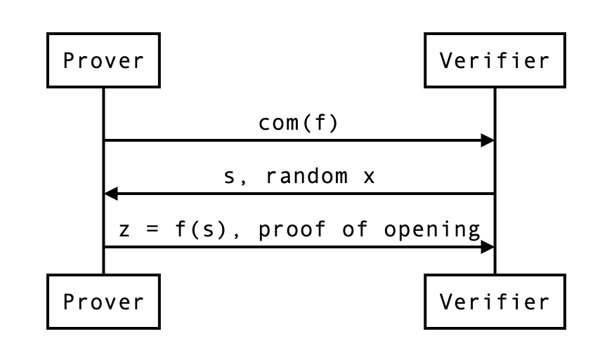
We can picture the protocol as follows:

1. The prover first sends a commitment to the polynomial $f$.
2. The verifier sends a point $s$, asking for the value $f(s)$. To help the prover perform a proof of correct evaluation, they also send a random challenge $x$. (NOTE: The verifier sends the random challenge $x$ ONLY AFTER they receive the $z=f(s)$)
3. The prover sends the result of the evaluation, $z$, as well as a proof.

Does that make sense? Of course what’s interesting to us is the proof, and how the prover uses that random $x$.

Reduced problem

First, the prover cuts everything in half. Then they use $x$ to construct linear combinations of these cuts:

• $\overrightarrow{a^{\prime }}=x^{-1}\left(\begin{array}{c}{a}_1\\ a_2\end{array}\right)+x\left(\begin{array}{c}{a}_3\\ a_4\end{array}\right)$
• $\overrightarrow{b^{\prime }}=x\left(\begin{array}{c}{b}_1\\ b_2\end{array}\right)+x^{-1}\left(\begin{array}{c}{b}_3\\ b_4\end{array}\right)$
• $\overrightarrow{G^{\prime }}=x\left(\begin{array}{c}{G}_1\\ G_2\end{array}\right)+x^{-1}\left(\begin{array}{c}{G}_3\\ G_4\end{array}\right)$

This is how the problem is reduced to $⟨\overrightarrow{a^{\prime }},\overrightarrow{b^{\prime }}⟩=z^{\prime }$.

At this point, the prover can send $\overrightarrow{a^{\prime }}$, $\overrightarrow{b^{\prime }}$, and $z^{\prime }$ and the verifier can check if indeed $⟨\overrightarrow{a^{\prime }},\overrightarrow{b^{\prime }}⟩=z^{\prime }$. But that wouldn’t make much sense would it? Here we also want:

• a proof that proving that statement is the same as proving the previous statement ($⟨\vec{a},\vec{b}⟩=z$)
• a way for the verifier to compute $z^{\prime }$ and $b^{\prime }$ and $A^{\prime }$ (the new commitment) by themselves.

The actual proof

The verifier can compute $\overrightarrow{b^{\prime }}$ as they have everything they need to do so.

What about $A^{\prime }$, the commitment of $\overrightarrow{a^{\prime }}$ which uses the new $\overrightarrow{G^{\prime }}$ basis. It should be the following value:

$$\begin{array}{rl}\overrightarrow{A^{\prime }}=& ⟨\overrightarrow{a^{\prime }},\overrightarrow{G^{\prime }}⟩\\ =& (x^{-1}{a}_1+x{a}_3)(x{G}_1+x^{-1}{G}_3)+(x^{-1}{a}_2+x{a}_4)(x{G}_2+x^{-1}{G}_4)\\ =& A+x^{-2}(a_1{G}_3+a_2{G}_4)+x^2(a_3{G}_1+a_4{G}_2)\\ =& A+x^{-2}{L}_a+x^2{R}_a\end{array}$$

So to compute this new commitment, the verifier needs:

• the previous commitment $A$, which they already have
• some powers of $x$, which they can compute
• two curve points $L_a$ and $R_a$, which the prover will have to provide to them

What about $z^{\prime }$? Recall:

• $\overrightarrow{a^{\prime }}=\left(\begin{array}{c}{x}^{-1}{a}_1+x{a}_3\\ x^{-1}{a}_2+x{a}_4\end{array}\right)$
• $\overrightarrow{b^{\prime }}=\left(\begin{array}{c}x{b}_1+x^{-1}{b}_3\\ x{b}_2+x^{-1}{b}_4\end{array}\right)$

So the new inner product should be:

$$\begin{array}{rl}\overrightarrow{z^{\prime }}=& ⟨\overrightarrow{a^{\prime }},\overrightarrow{b^{\prime }}⟩\\ =& ⟨\left(\begin{array}{c}{x}^{-1}{a}_1+x{a}_3\\ x^{-1}{a}_2+x{a}_4\end{array}\right),\left(\begin{array}{c}x{b}_1+x^{-1}{b}_3\\ x{b}_2+x^{-1}{b}_4\end{array}\right)⟩\\ =& (a_1{b}_1+a_2{b}_2+a_3{b}_3+a_4{b}_4)+x^{-2}(a_1{b}_3+a_2{b}_4)+x^2(a_3{b}_1+a_4{b}_2)\\ =& z+x^{-2}(L_z)+x^2(R_z)\end{array}$$

Similarly to $A^{\prime }$, the verifier can recompute $z^{\prime }$ from the previous value $z$ and two scalar values $L_z$ and $R_z$ which the prover needs to provide.

So in the end, the proof has become:

• the vector $\overrightarrow{a^{\prime }}$ which is half the size of $\vec{a}$
• the $L_a,R_a$ curve points (around two field elements, if compressed)
• the $L_z,R_z$ scalar values

We can update our previous diagram:

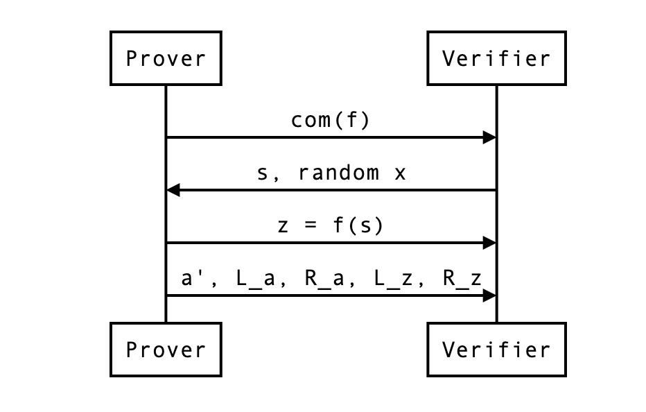
In our example, the naive proof was to reveal $\vec{a}$ which was 4 field elements. We are now revealing instead 2 + 2 + 2 = 6 field elements. This is not great, but if $\vec{a}$ was much larger (let’s say 128), the reduction in half would still be of 64 + 2 + 2 = 68 field elements. Not bad no? We can do better though…

The HALO optimization

The HALO optimization is similar to the bulletproof optimization, but it further reduces the size of our proof, so I’ll explain that directly.

With the HALO optimization, the prover translates the problem into the following:

$$C=A+zU=⟨\vec{a},\vec{G}⟩+⟨\vec{a},\vec{b}⟩U$$

This is simply a commitment of $\vec{a}$ and $z$.

A naive proof is to reveal $\vec{a}$ and let the verifier check that it is a valid opening of the following commitment. Then, that commitment will be reduced recursively to commitments of the same form.

$$C^{\prime }=A^{\prime }+z^{\prime }U=⟨\overrightarrow{a^{\prime }},\overrightarrow{G^{\prime }}⟩+⟨\overrightarrow{a^{\prime }},\overrightarrow{b^{\prime }}⟩U$$

The whole point is that the reduction proofs will be smaller than our previous bootleproof-inspired protocol.

How does the reduction proof work? Notice that this is the new commitment:

$$\begin{array}{rl}{C}^{\prime }=& ⟨\overrightarrow{a^{\prime }},\overrightarrow{G^{\prime }}⟩+⟨\overrightarrow{a^{\prime }},\overrightarrow{b^{\prime }}⟩U\\ =& [A+x^{-2}{L}_a+x^2{R}_a]+[z+x^{-2}(L_z)+x^2(R_z)]U\end{array}$$

This is simply from copy/pasting the equations from the previous section. This can be further reduced to:

$$C^{\prime }=C+x^{-2}(L_a+L_{z}U)+x^2(R_a+R_{z}U)$$

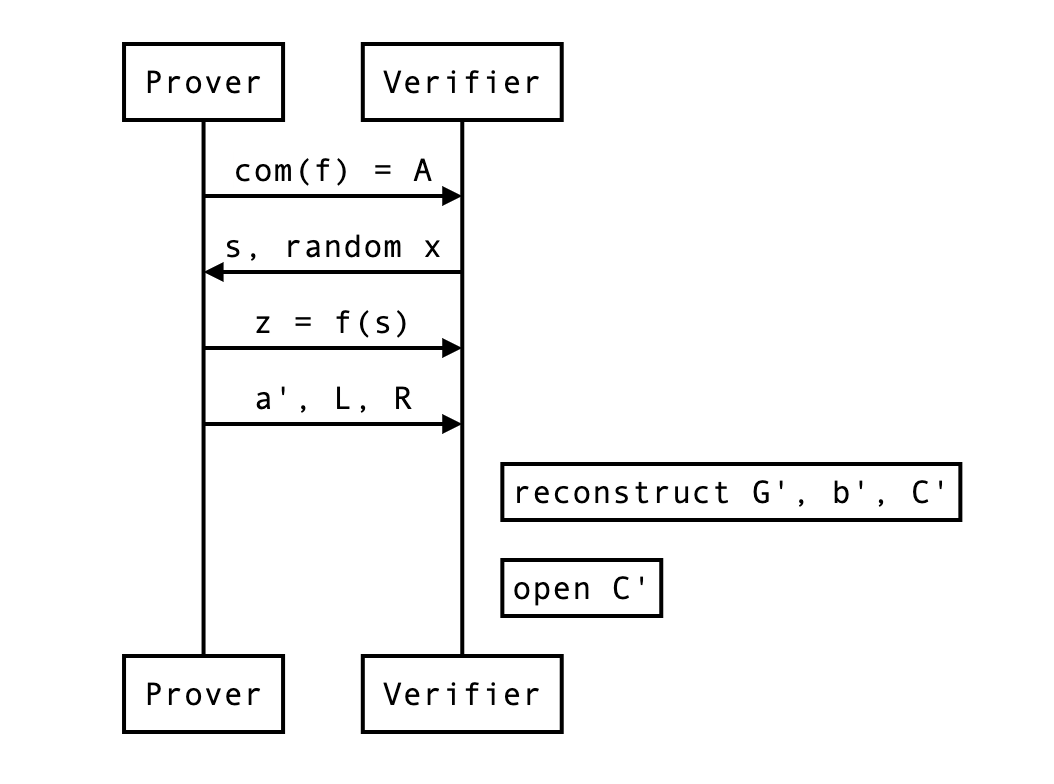
And now you see that the verifier now only needs, in addition to $\overrightarrow{a^{\prime }}$, two curve points (~ 2 field elements):

• $L=L_a+L_{z}U$
• $R=R_a+R_{z}U$

this is in contrast to the 4 field elements per reduction needed without this optimization. Much better right?

At the end of a round (or the protocol) the verifier can compute the expected commitment $C^{\prime }$ as such:

$$C^{\prime }=C+x^{-2}L+x^{2}R$$

and open it by computing the following and checking it is indeed equal to $C^{\prime }$:

$$⟨\overrightarrow{a^{\prime }},\overrightarrow{G^{\prime }}⟩+⟨\overrightarrow{a^{\prime }},\overrightarrow{b^{\prime }}⟩U$$

For this, the verifier needs to recompute $\overrightarrow{G^{\prime }}$ and $\overrightarrow{b^{\prime }}$ by themselves, which they can as they have all the necessary information. We can update our previous diagram:

What about zero-knowledge?

Didn’t we forget something? Oh right, we’re sending $a^{\prime }$ in clear, a single element that will leak some information about the original vector $\vec{a}$ (as it is a linear combination of that original vector).

The simple solution is to alter our pedersen commitment to make it hiding on top of being binding:

$$C=A+zU+rH=⟨\vec{a},\vec{G}⟩+⟨\vec{a},\vec{b}⟩U+rH$$

where H is another generator we don’t know the discrete logarithm of, and $r$ is a random scalar value generated by the prover to blind the commitment.

But wait, each $L$ and $R$ also leaks some! As they are also made from the original secret vector $\vec{a}$. Remember, $L=L_a+L_{z}U$ No worries, we can perform the same treatment on that curve point and blind it like so:

• $L=L_a+L_{z}U+r_{L}H$
• $R=R_a+R_{z}U+r_{R}H$

In order to open the final commitment, the verifier first recomputes the expected commitment as before:

$$C^{\prime }=C+x^{-2}L+x^{2}R$$

then use $\overrightarrow{a^{\prime }}$ and the final blinding value $r^{\prime }$ sent by the prover (and composed of $r$ and all the rounds’ $r_L$ and $r_R$), as well as reconstructed $\overrightarrow{G^{\prime }}$ and $\overrightarrow{b^{\prime }}$ to open the commitment:

$$⟨\overrightarrow{a^{\prime }},\overrightarrow{G^{\prime }}⟩+⟨\overrightarrow{a^{\prime }},\overrightarrow{b^{\prime }}⟩U+r^{\prime }H$$

with $r^{\prime }$ being equal to something like $r+{\sum }_i(r_{Li}+r_{Ri})$

At this point, the protocol requires the sender to send:

• 2 curve points $L$ and $R$ per rounds
• 1 scalar value $a^{\prime }$ for the final opening
• 1 blinding (scalar) value $r^{\prime }$ for the final opening

But wait… one last thing. In this protocol the prover is revealing $\overrightarrow{a^{\prime }}$, and even if they were not, by revealing $r^{\prime }$ they might allow someone to recompute $\overrightarrow{a^{\prime }}$… The HALO paper contains a generalized Schnorr protocol to open the commitment without revealing $\overrightarrow{a^{\prime }}$ nor $r^{\prime }$.

from Vanishree:

• So in general the more data we send the more randomness we need to ensure the private aspects are hidden, right
• The randomness in a commitment is because we are sending the commitment elements
• The random elements mixed with the polynomial (in the new zkpm technique) is because we send evaluations of the polynomial at zeta and zeta omega later
• Zk in Schnorr opening is because we reveal the opening values

where can I find a proof? perhaps appendix C of https://eprint.iacr.org/2017/1066.pdf

The real protocol, and a note on non-interactivity

Finally, we can look at what the real protocol end up looking at with $lo{g}_2(n)$ rounds of reduction followed by a commitment opening.

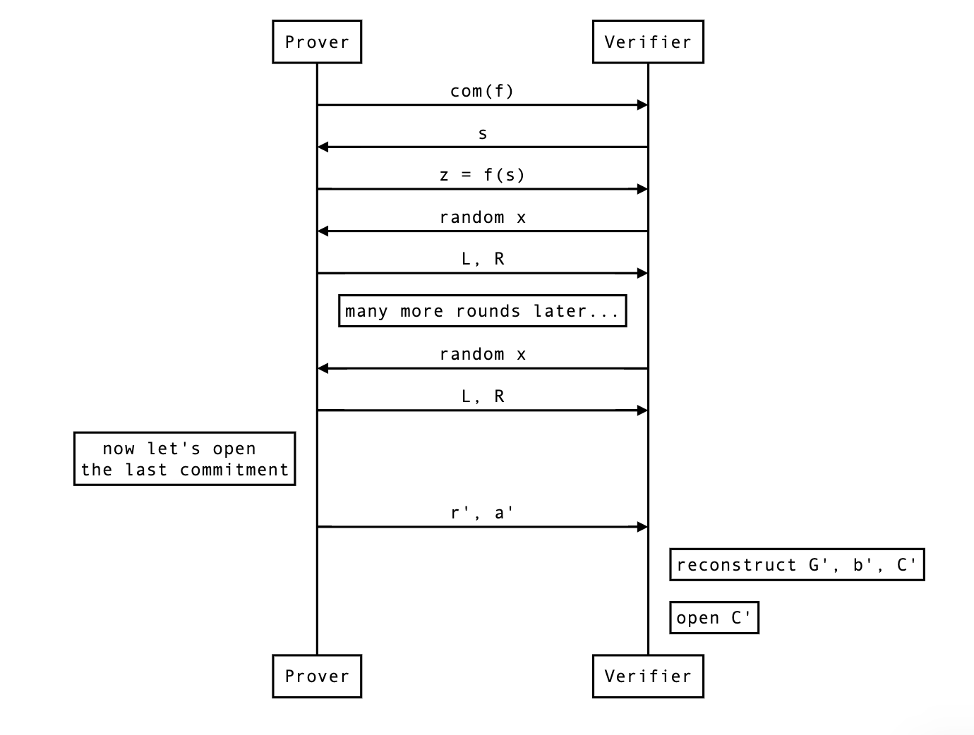
So far the protocol was interactive, but you can make it non-interactive by simply using the Fiat-Shamir transformation. That’s all I’ll say about that.